Plot calibration of dynamic risk predictions

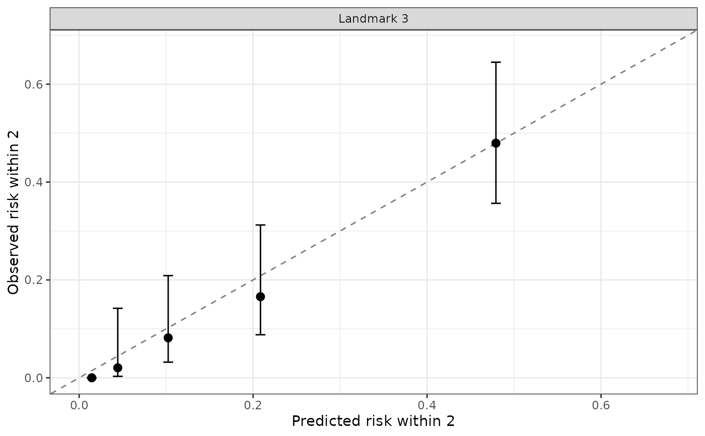
Checks whether the predicted risks are numerically right, not just well ranked. At each landmark s in prediction_time, every subject in data_predict_all still event-free at s gets a predicted risk from predictRisk of an event in (s, s + horizon], using only their longitudinal history up to s. The subjects are split into n_groups groups of about equal size by predicted risk, and for each group the mean predicted risk (horizontal axis) is plotted against the observed risk (vertical axis): one minus the Kaplan–Meier estimate at s + horizon or, with competing risks, the Aalen–Johansen cumulative incidence of that event type, both of which account for censoring, with 95\ intervals. Points on the diagonal mean the predictions are well calibrated; points below it mean the model overestimates the risk, above it that it underestimates it.

Evaluating on the data the sub-models were fit on gives an optimistic (apparent) calibration; pass held-out validation data in data_predict_all when available.

For an interval-censored fit (experimental), the observed risk of a group is a nonparametric (Turnbull-type) estimate from the subjects' intervals, left-truncated at each subject's last visit up to the landmark – with competing risks, the cumulative incidence estimate of Hudgens, Satten and Longini (2001) – so it estimates the same quantity predictRisk() predicts, without using the model. Within an interval the timing of the event is not identified, so the estimate is less precise than with exact times, and no confidence interval is drawn. In simulations it was unbiased when the visits were at most about horizon apart, but with visits further apart than horizon the window mostly falls inside the subjects' intervals and the observed risk of the higher-risk groups was much too high (up to +0.27 with visits every 2–6 years and a 2-year window). An observed risk computed from the model's own posterior was more precise, but followed the predictions of a deliberately miscalibrated model instead of the truth, so it is not offered.

Usage

calibrationPlot(
  data_predict_all,
  long_fit_all,
  survival_fit_all,
  prediction_time,
  horizon,
  time_variable,
  survival_variable_all,
  survival_trans_function,
  n_groups = 10,
  bandcount1 = "auto",
  bandcount2 = "auto"
)

Arguments

data_predict_all

The evaluation data, in the same format as for predictRisk: a list of long-format data.frames, one per longitudinal outcome (or a single data.frame used for all). Unlike for predictRisk(), it must also contain each subject's observed outcome: the survival time and status variables of survival_fit_all's Cox formula and, with competing risks, the event type variable of its form_conditional_cr. The outcome is taken from the first data frame and is hidden from predictRisk().

long_fit_all

A longitudinalSub.BJM object from longitudinalSub.

survival_fit_all

A survivalSub.BJM object from survivalSub.

prediction_time

A vector of landmark times.

horizon

The prediction horizon (a single positive number): the window after each landmark in which events are counted.

time_variable

The name of the time variable in the linear mixed models.

survival_variable_all, survival_trans_function

As for predictRisk.

n_groups

Number of risk groups per landmark. Default 10 (deciles); fewer groups give more stable observed risks in small data.

bandcount1, bandcount2

As for predictRisk; passed to it at each landmark.

Value

A ggplot object with one panel per landmark (and, with competing risks, per event type). Its data element is a data.frame with one row per risk group, and columns landmark, cause, group, predicted, observed, lower, upper, n (subjects in the group) and n_cases (events of that type observed in the window).

Examples

# \donttest{
data(pbc3)
survival_fit_all <- survivalSub(pbc3[!duplicated(pbc3$id), ],
                                Surv(years, status3) ~ age + sex, NULL)
long_sub_fixed <- list("long1" = serBilir ~ year + age + sex + years)
long_sub_random <- list("long1" = ~ year | id)
long_fit_all <- longitudinalSub(list(pbc3[pbc3$status3 == 1, ]),
                                long_sub_fixed, long_sub_random)
trans <- survivalTrans(c(1, 3, 5, 7))

# apparent calibration on the fitting data: 3-year landmark, 2-year window
calibrationPlot(pbc3, long_fit_all, survival_fit_all,
  prediction_time = 3, horizon = 2, time_variable = "year",
  trans$survival_variable_all, trans$survival_trans_function, n_groups = 5)

# }