Digital twins

A patient’s digital twin is a model of that patient that is updated as their data arrive and can be run forward to show how they may fare. For longitudinal clinical data, the twin has to forecast two things together: how the patient’s biomarkers will evolve, and when an event (and which event) will happen. The backward joint model does both, and simulateTrajectory() turns a fitted model into a twin: it draws complete futures for a patient, conditional on everything measured so far.

A digital twin needs	In BJM
a model of the individual patient	the joint model with the patient’s random effects
to be synchronized with new data	conditioning on the history up to prediction_time
to forecast the patient’s state	draws of future biomarker values and of the event time and type
to quantify uncertainty	many draws per patient (n_sim)
to describe patients not seen yet	a patient with no measurements is drawn from their covariates alone

This article shows four uses on the pbc3 data: a twin that is updated at each visit, questions answered from the twin’s draws, virtual patients, and twins as a prognostic covariate in a randomized trial. The twin is a statistical, predictive model: it forecasts outcomes as observed in the data it was fit on, and is not a mechanistic or causal model of the disease.

library(BJM)
library(ggplot2)
data(pbc3)

We fit the sub-models as in vignette("BJM-intro"): a Cox model for death or transplantation (status3), a logistic model for which of the two occurred (status4: 0 death, 1 transplantation), and serum bilirubin (serBilir, log scale) and albumin as biomarkers.

survival_fit_all <- survivalSub(
  pbc3[!duplicated(pbc3$id), ],
  form_marginal_surv = Surv(years, status3) ~ age + sex,
  form_conditional_cr = status4 ~ years + age + sex
)

long_sub_fixed <- list(
  "serBilir" = serBilir ~ year + age + sex + years + years * year,
  "albumin"  = albumin  ~ year + age + sex + years + years * year
)
long_sub_random <- list("serBilir" = ~ year | id, "albumin" = ~ year | id)
long_fit_all <- longitudinalSub(pbc3[pbc3$status3 == 1, ], long_sub_fixed, long_sub_random)

trans <- survivalTrans(c(1, 3, 5, 7))

A twin that is updated at each visit

Patient 2 was followed for 14 years. We build their twin three times, at years 1, 3 and 5, each time from the measurements taken so far, and draw 500 futures over the next five years. The event time and type are set to NA: at each of these times they are not known yet.

patient <- pbc3[pbc3$id == 2, ]

twin_at <- function(landmark) {
  history <- patient[patient$year <= landmark, ]
  history$years <- NA
  history$status4 <- NA
  sims <- simulateTrajectory(history, long_fit_all, survival_fit_all,
                             prediction_time = landmark,
                             times = seq(landmark, landmark + 5, by = 0.25),
                             time_variable = "year",
                             trans$survival_variable_all, trans$survival_trans_function,
                             n_sim = 500, seed = 1)
  sims$landmark <- landmark
  as.data.frame(sims)
}
twins <- do.call(rbind, lapply(c(1, 3, 5), twin_at))

simulateTrajectory() returns one row per draw and time, so any summary is a few lines of ordinary R. Each draw’s event time is repeated on all of its rows; keeping the first row of each draw gives one row per future. The twin’s risk of an event within three years grows as the patient’s bilirubin rises:

futures <- twins[!duplicated(twins[c("landmark", "sim")]), ]
aggregate(cbind(risk_3_years = event == 1 & event_time <= landmark + 3) ~ landmark,
          data = futures, FUN = mean)
#>   landmark risk_3_years
#> 1        1        0.036
#> 2        3        0.102
#> 3        5        0.212

The forecast bilirubin, with every measurement the patient actually had. Filled points are the ones the twin was built from; open points were measured later, and show how the twin’s forecasts compare with what happened.

bands <- aggregate(serBilir ~ landmark + year, data = twins,
                   FUN = function(v) quantile(v, c(0.05, 0.5, 0.95)))
bands <- do.call(data.frame, bands)
names(bands)[3:5] <- c("lower", "median", "upper")

measured <- merge(patient[c("year", "serBilir")], data.frame(landmark = c(1, 3, 5)))
measured$used <- ifelse(measured$year <= measured$landmark, "used by the twin", "measured later")

ggplot(bands, aes(x = year)) +
  geom_ribbon(aes(ymin = lower, ymax = upper), fill = "#2166AC", alpha = 0.2) +
  geom_line(aes(y = median), color = "#2166AC", linewidth = 1) +
  geom_point(data = measured, aes(y = serBilir, shape = used), size = 2) +
  scale_shape_manual(values = c("used by the twin" = 16, "measured later" = 1), name = NULL) +
  geom_vline(aes(xintercept = landmark), linetype = "dashed", color = "grey50") +
  facet_wrap(~ landmark, labeller = label_both) +
  ylab("serBilir") + theme_bw() + theme(legend.position = "bottom")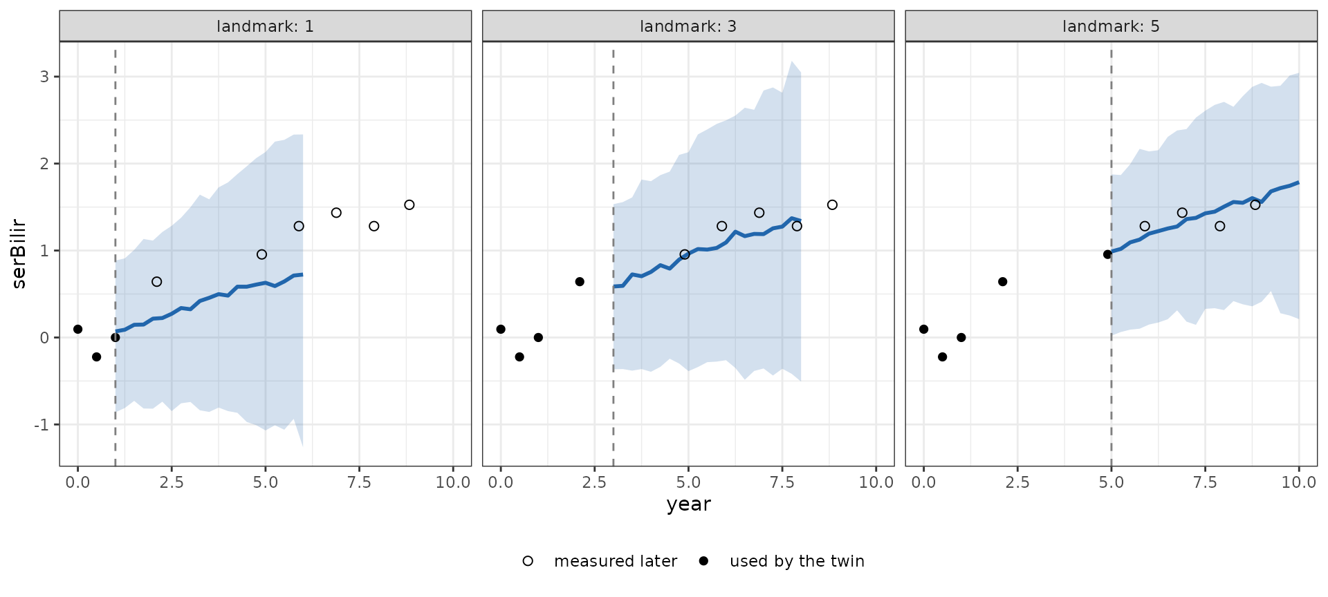

plot(sims) and plot(sims, which = "event") draw a single twin directly; see Plotting with BJM.

Asking the twin questions

Because the twin is a set of draws rather than a few summary numbers, it answers questions no single prediction function was written for. Using the twin built at year 5:

at5 <- twins[twins$landmark == 5, ]
futures5 <- at5[!duplicated(at5$sim), ]

# median time to death or transplantation, among the futures with an event
# within follow-up
median(futures5$event_time[futures5$event == 1])
#> [1] 9.253643

# probability of being event-free at year 8 with bilirubin above 2
# (serBilir is on the log scale, so this is above about 7.4 mg/dL)
mean(sapply(split(at5, at5$sim), function(d) {
  at8 <- d[d$year == 8, ]
  !is.na(at8$serBilir) && at8$serBilir > 2
}))
#> [1] 0.18

# probability that albumin falls below 2.8 before any event, within 3 years
mean(sapply(split(at5, at5$sim), function(d) {
  window <- d[d$year <= 8 & !is.na(d$albumin), ]
  any(window$albumin < 2.8)
}))
#> [1] 0.708

Covariates after the last visit

To forecast the biomarkers at a future time, the twin needs the patient’s covariates at that time. By default it carries forward the values in the patient’s last row. In this article’s models the covariates are age at entry and sex, which do not change, so carrying them forward is exact.

A covariate that does change, such as ascites or a change of treatment, is not forecast by the model, and carrying it forward assumes it stays as it was last seen. future_covariates sets a different path: each row gives covariate values that apply from its time on, until a later row changes them. For example, data.frame(year = 6, ascites = "Yes") would set ascites from year 6 on, in a model with ascites as a covariate. With an id column the rows apply to that patient only.

With this article’s models, future_covariates can serve as a sensitivity check of how much the forecast depends on a covariate. Here patient 2’s year-5 twin is drawn again with age set 10 years higher from year 7 on. This is not a realistic scenario, since age at entry cannot change, but it shows how the path enters the forecast.

history5 <- patient[patient$year <= 5, ]
history5$years <- NA
history5$status4 <- NA

draw_twin <- function(future_covariates = NULL) {
  simulateTrajectory(history5, long_fit_all, survival_fit_all,
                     prediction_time = 5, times = 5:10, time_variable = "year",
                     trans$survival_variable_all, trans$survival_trans_function,
                     n_sim = 500, future_covariates = future_covariates, seed = 1)
}
as_measured <- draw_twin()
older_from_7 <- draw_twin(data.frame(year = 7, age = history5$age[1] + 10))

# median forecast bilirubin at each year, among the draws still event-free
cbind(as_measured = tapply(as_measured$serBilir, as_measured$year, median, na.rm = TRUE),
      older_from_7 = tapply(older_from_7$serBilir, older_from_7$year, median, na.rm = TRUE))
#>    as_measured older_from_7
#> 5    0.9702453    0.9702453
#> 6    1.1620662    1.1620662
#> 7    1.3584893    1.2417347
#> 8    1.4929772    1.3762226
#> 9    1.7231421    1.6063875
#> 10   1.6938166    1.5770620

The forecasts agree up to year 6 and differ from year 7 on, by the model’s age coefficient times 10. The history the twin conditions on is the same in both, so the drawn event times and random effects are the same too: future_covariates changes only the forecast biomarker values. Comparing covariate paths in this way compares the outcomes the model associates with them, not the causal effect of changing them.

Virtual patients

A twin can also be built for a patient who has not been measured at all, from baseline covariates alone, with the biomarkers set to NA. Here two virtual patients, aged 40 and 70, otherwise alike.

virtual <- data.frame(id = c("age 40", "age 70"), year = 0, age = c(40, 70), sex = 1,
                      serBilir = NA, albumin = NA)
virtual_sims <- simulateTrajectory(virtual, long_fit_all, survival_fit_all,
                                   prediction_time = 0, times = 0:10, time_variable = "year",
                                   trans$survival_variable_all, trans$survival_trans_function,
                                   n_sim = 1000, seed = 1)
virtual_futures <- virtual_sims[!duplicated(virtual_sims[c("id", "sim")]), ]
aggregate(cbind(death_5_years = event == 1 & status4 == 0 & event_time <= 5,
                transplant_5_years = event == 1 & status4 == 1 & event_time <= 5,
                event_free_14_years = event == 0) ~ id,
          data = virtual_futures, FUN = mean)
#>       id death_5_years transplant_5_years event_free_14_years
#> 1 age 40         0.167              0.109               0.387
#> 2 age 70         0.420              0.002               0.207

The cumulative incidence of each event type, computed from the draws:

grid <- seq(0, attr(virtual_sims, "max_event_time"), length.out = 200)
incidence <- do.call(rbind, lapply(split(virtual_futures, virtual_futures$id), function(d) {
  do.call(rbind, lapply(c(death = 0, transplantation = 1), function(type) {
    data.frame(id = d$id[1], time = grid,
               event = if (type == 0) "death" else "transplantation",
               incidence = vapply(grid, function(t)
                 mean(d$event == 1 & d$status4 == type & d$event_time <= t), numeric(1)))
  }))
}))

ggplot(incidence, aes(x = time, y = incidence, color = id)) +
  geom_line(linewidth = 1) +
  facet_wrap(~ event) +
  labs(x = "year", y = "Cumulative incidence", color = NULL) +
  theme_bw()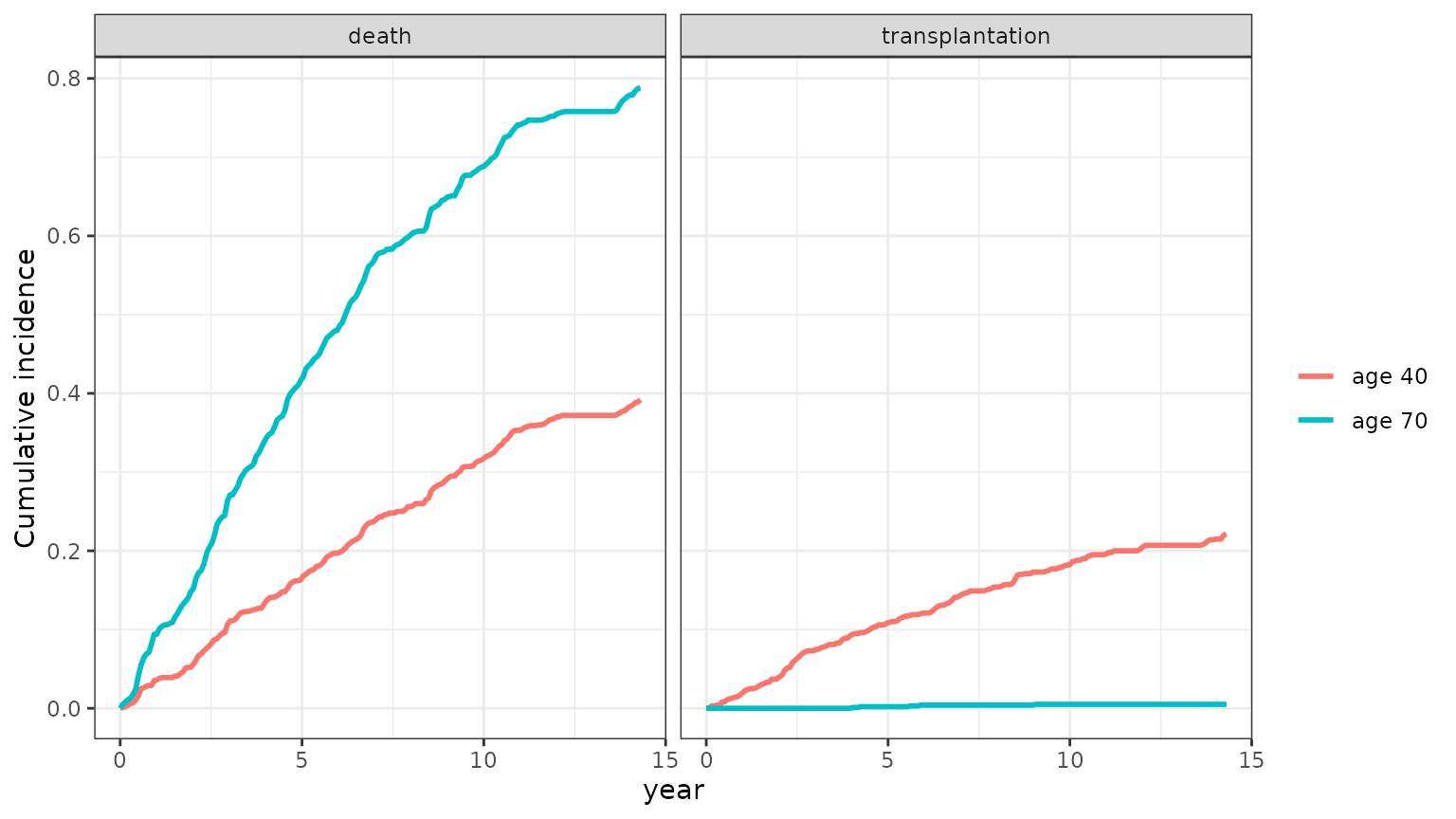

The difference between the two reflects how age is associated with the outcomes in pbc3; it is not the effect of being older, and a virtual patient is only as realistic as the covariates it is given. To build a synthetic cohort, give each virtual patient covariates resampled from the population of interest, as in Plotting with BJM.

Twins in a randomized trial

pbc3 comes from a randomized trial of D-penicillamine against placebo (drug). A common use of digital twins in trials is to predict each participant’s outcome from their baseline data, and to adjust the treatment comparison for that prediction, which reduces the variance of the estimated treatment effect without biasing it, since the prediction uses only data from before randomization (the idea behind PROCOVA).

The outcome here is bilirubin at the visit near year 2, for the 220 participants who had one. Each participant’s twin is built from their baseline measurements alone (the event time is unknown at baseline), and its prediction is the mean of 200 draws of their bilirubin at year 2. With truncate = FALSE the draws are not cut off at the drawn event time, so the prediction is of the biomarker itself rather than of it among the draws still event-free.

visit_2y <- pbc3[pbc3$year > 1.5 & pbc3$year < 2.5, ]
visit_2y <- visit_2y[!duplicated(visit_2y$id), c("id", "drug", "serBilir")]
names(visit_2y)[3] <- "serBilir_2y"

baseline <- pbc3[pbc3$year == 0 & pbc3$id %in% visit_2y$id, ]
baseline$years <- NA
baseline$status3 <- NA
baseline$status4 <- NA

trial_twins <- simulateTrajectory(baseline, long_fit_all, survival_fit_all,
                                  prediction_time = 0, times = 2, time_variable = "year",
                                  trans$survival_variable_all, trans$survival_trans_function,
                                  n_sim = 200, truncate = FALSE, seed = 1)
prognosis <- aggregate(cbind(twin_serBilir = serBilir) ~ id, data = trial_twins, FUN = mean)
trial <- merge(visit_2y, prognosis, by = "id")

cor(trial$twin_serBilir, trial$serBilir_2y)
#> [1] 0.8127169

The treatment effect on bilirubin at year 2, without and with the twin’s prediction as a covariate:

unadjusted <- lm(serBilir_2y ~ drug, data = trial)
adjusted <- lm(serBilir_2y ~ drug + twin_serBilir, data = trial)
rbind(unadjusted = coef(summary(unadjusted))["drugD-penicil", ],
      twin_adjusted = coef(summary(adjusted))["drugD-penicil", ])
#>                  Estimate Std. Error    t value  Pr(>|t|)
#> unadjusted    -0.03056175 0.15509068 -0.1970573 0.8439663
#> twin_adjusted -0.07962104 0.09045106 -0.8802666 0.3796888

# sample size the unadjusted analysis would need for the same precision,
# relative to the trial's
(coef(summary(unadjusted))["drugD-penicil", "Std. Error"] /
   coef(summary(adjusted))["drugD-penicil", "Std. Error"])^2
#> [1] 2.939978

Both analyses agree that D-penicillamine has no clear effect on bilirubin, as the trial found; the adjusted one estimates it with a much smaller standard error, which in a new trial would translate into fewer patients for the same power. Two caveats apply to this illustration:

• The twins here were fit on the same pbc3 data, including the trial’s outcomes. In practice the model is fit on historical data, such as earlier trials or registries, and frozen before the trial starts.
• Most of the gain here comes from baseline bilirubin, which the twin carries forward; adjusting for it directly gives a similar standard error. A twin earns its keep when it combines many baseline biomarkers and covariates, measured irregularly, into one prediction.

What the twin assumes

The twin inherits the assumptions of the fitted model, and adds a few of its own (see ?simulateTrajectory for details):

• Fixed parameters. The draws use the estimated parameters as if they were known, so the spread of the futures reflects differences between patients and measurement error, not uncertainty in the estimates.
• Follow-up limits. Event times after the last follow-up time of the data (max_event_time) are reported as event-free through it, rather than extrapolated.
• Carried-forward covariates. Future biomarker values use each covariate’s last value, unless future_covariates gives another path.
• Who the longitudinal model describes. The longitudinal sub-model is fit on patients with an event, so it describes trajectories leading to an event; a twin of a patient who will be event-free for a long time is approximated by one whose event comes at the end of follow-up.