Simulate future trajectories from the backward joint model

Draws n_sim complete futures for each patient from the fitted backward joint model, conditional on the patient's longitudinal history up to prediction_time and on being event-free at prediction_time: an event time (and, with competing risks, an event type), and the values of every biomarker at the requested times. Where predictRisk and predictLongitudinal summarize the predictive distribution, this returns samples from it, so it can be used to generate synthetic patients or to propagate the prediction into any other quantity (e.g. a patient's "digital twin" under the fitted model).

Each draw follows the model's factorization \(f(T, D)\, f(Y \mid T, D)\):

\((T, D)\) is drawn from its posterior given the history, proportional to \(f(Y_{hist} \mid T, D)\, f(D \mid T)\, f(T)\) restricted to \(T > \) prediction_time, evaluated on the same integration grid as predictRisk's denominator;
the random effects \(b\) are drawn from their Gaussian posterior given the history and the drawn \((T, D)\);
the biomarkers at times are drawn from the longitudinal sub-model given \((T, D, b)\), adding residual error.

A patient with no non-missing biomarker measurement up to prediction_time (e.g. a single baseline row with the biomarkers set to NA) is simulated from the model's prior given their baseline covariates, i.e. as a new synthetic patient.

Usage

simulateTrajectory(
  data_predict_all,
  long_fit_all,
  survival_fit_all,
  prediction_time,
  times,
  time_variable,
  survival_variable_all,
  survival_trans_function,
  n_sim = 100,
  bandcount2 = 100,
  max_event_time = NULL,
  truncate = TRUE,
  future_covariates = NULL,
  seed = NULL
)

Arguments

data_predict_all: This involves a collection of data.frame objects for dynamic prediction, each corresponding to a distinct longitudinal outcome. These data frames should contain the variables specified in long_sub_fixed and long_sub_random. Utilizing a list structure allows for the incorporation of multiple longitudinal outcomes, each potentially following different measurement protocols. In instances where all longitudinal outcomes are recorded at identical time points across patients, a singular data.frame object may be used in a list. Alternatively, a single bare data.frame (not wrapped in a list) may be supplied directly; it is then reused for every longitudinal outcome. It is presumed that each data frame is structured in a long format.
long_fit_all: Outputs from the model fitting process using the nlme package, encompassing the results and parameters obtained from the analysis.
survival_fit_all: Results and parameters generated from the model fitting procedure, utilizing the coxph function. These outputs include the comprehensive findings and variables derived from the analysis.
prediction_time: Time used to make the prediction.
times: Numeric vector of times (on the scale of time_variable) at which to simulate the biomarkers, each at least prediction_time.
time_variable: The name of time variable in linear mixed model.
survival_variable_all: The name of the transformed time-to-event outcomes variable.
survival_trans_function: The transformation function used for time-to-event outcomes, in the order of survival_variable_all.
n_sim: Number of futures to draw per patient.
bandcount2: The number of intervals the event-time distribution after prediction_time is discretized into (see Details and predictRisk).
max_event_time: Event times beyond this are reported as event-free through it, and the model is evaluated at it in their place (see Details). Defaults to NULL, the last follow-up time of the data survivalSub() was fit on; Inf turns this off.
truncate: If TRUE, biomarker values at or after the drawn event time are NA (see Details).
future_covariates: Optional data frame of covariate values at future times: a time_variable column, one column per covariate to set, and optionally the patient id column (named as in long_sub_random) to set them per patient; without it, every row applies to every patient. It cannot set the biomarkers or the event time or type. See Details.
seed: Optional integer seed, for reproducible draws. The caller's random number stream is left unchanged.

Value

A data frame of class "simulateTrajectory.BJM", with one row per patient, draw and element of times, and columns: the patient id (named as in long_sub_random); sim, the draw number; time_variable; event_time, the drawn event time, or max_event_time if the event comes after it; event, 1 if the event occurs at event_time and 0 if the patient is event-free through it; with competing risks, the drawn event type (named as the response of form_conditional_cr, with the same 0/1 coding, and NA when event is 0); and one column per biomarker, named by its response variable (an ordered factor, with the fitted categories as levels, for an ordinal biomarker). Attributes "prediction_time", "times" and "max_event_time" record the values used, and "history" the continuous biomarker measurements conditioned on (for plot.simulateTrajectory.BJM).

Details

The event time is drawn on the grid of bandcount2 intervals that predictRisk integrates over (each holding about the same share of the conditional survival probability, with an extra edge at max_event_time): an interval is drawn with its posterior probability, the model is evaluated at its midpoint, and the event time reported is uniform within it, so that summaries of the drawn event times (e.g. the share before a given time) are not biased by rounding to the midpoints.

Past the last follow-up time of the data survivalSub() was fit on, the event-time distribution rests on an extrapolated baseline hazard and the longitudinal sub-model's mean on event times it was never fit on; drawn from a patient's prior (no history), a large share of event times can land there, with implausible biomarker values. So an event time beyond max_event_time (by default that last follow-up time) is reported as event-free through max_event_time (event = 0, event_time = max_event_time), and both the history's likelihood and the simulated biomarkers use T = max_event_time in its place, i.e. a patient whose event comes after follow-up is assumed to follow the trajectory of one whose event comes at its end. max_event_time = Inf turns this off and reproduces the event-time distribution predictRisk integrates over.

The biomarkers at times are evaluated with the covariates of the patient's last row in data_predict_all (with time_variable set to each element of times), so a time-varying covariate is carried forward at its last value, unless future_covariates says otherwise. Each row of future_covariates sets the covariates in its columns from its time_variable on, until a later row changes them: a time in times takes the covariates of the last row at or before it, and those of the patient's last row in data_predict_all for anything that row does not set. The history, and so the posterior of the event time and random effects, is unaffected. A covariate that is a known function of time (such as current age) is better written into the model formula as one (e.g. I(age + year)), so that it is updated without future_covariates. Comparing draws under different future_covariates compares the outcomes the model associates with those covariate paths; it is not a causal effect of changing them.

The backward model describes the biomarkers before the event. With truncate = TRUE (the default) a value at a time at or after the drawn (or censored) event time is NA; with truncate = FALSE it is still drawn from the sub-model, which is the quantity whose density predictLongitudinal returns.

An ordinal biomarker (see longitudinalSubCopula) is the discretization of a latent Gaussian score by the fitted thresholds, and is simulated that way: its latent score is drawn like a continuous biomarker (with unit residual variance) and cut into categories. In the history it is known only to have fallen between the thresholds bracketing its observed category: its contribution to the likelihood of \((T, D)\) is a multivariate normal box probability, computed by Monte Carlo as in predictRisk, and the random effects are drawn by first drawing the history's latent scores from their truncated multivariate normal distribution given the continuous measurements (by rejection, or by Gibbs sampling when few proposals fall in the box), and then the random effects given those scores. Supply seed for reproducible draws.

Examples

# \donttest{
data(pbc3)

survival_fit_all = survivalSub(pbc3[!duplicated(pbc3$id), ],
                               Surv(years, status3) ~ age + sex, NULL)

long_sub_fixed = list(
  "long1" = serBilir ~ year + age + sex + (years) + (years) * year,
  "long2" = albumin ~ year + age + sex + (years) + (years) * year)
long_sub_random = list("long1" = ~ year | id, "long2" = ~ year | id)
data_fit_all = list(pbc3[pbc3$status3 == 1, ], pbc3[pbc3$status3 == 1, ])
long_fit_all = longitudinalSub(data_fit_all, long_sub_fixed, long_sub_random)

trans = survivalTrans(c(1, 3, 5, 7))

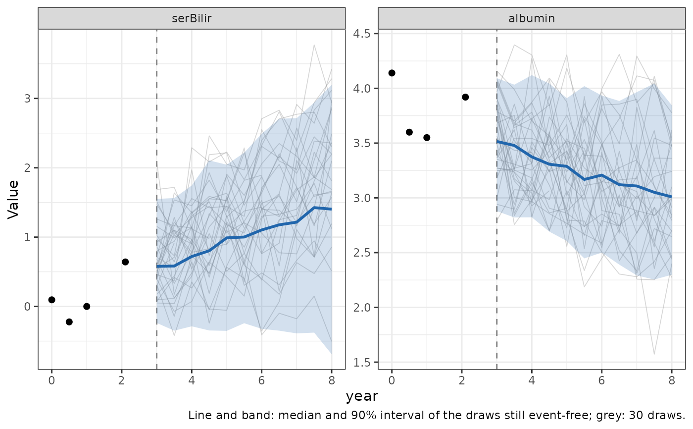
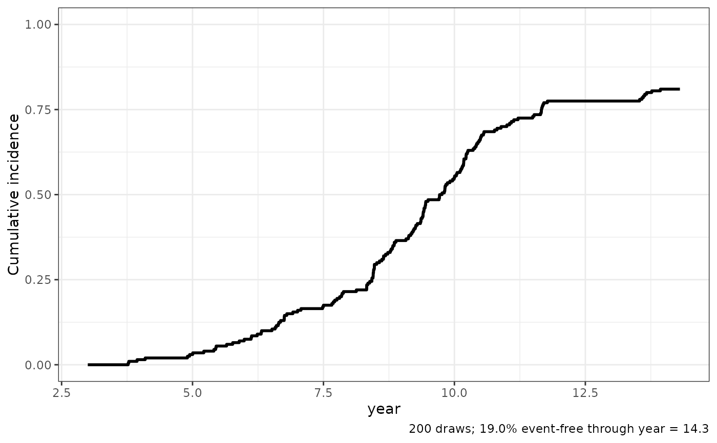
# Patient 2's history up to year 3: 200 possible futures over years 3-8
history = pbc3[pbc3$id == 2 & pbc3$year <= 3, ]
sims = simulateTrajectory(list(history, history), long_fit_all, survival_fit_all,
                          prediction_time = 3, times = seq(3, 8, by = 0.5),
                          time_variable = "year", trans$survival_variable_all,
                          trans$survival_trans_function, n_sim = 200, seed = 1)
head(sims)
#>   id sim year event_time event  serBilir  albumin
#> 1  2   1  3.0   10.38897     1 0.4707228 3.352258
#> 2  2   1  3.5   10.38897     1 1.6383372 3.308015
#> 3  2   1  4.0   10.38897     1 1.3522315 3.253805
#> 4  2   1  4.5   10.38897     1 1.5869380 3.428172
#> 5  2   1  5.0   10.38897     1 1.5204490 3.151635
#> 6  2   1  5.5   10.38897     1 2.2175576 2.982109

# Covariates after the last row are carried forward unless
# future_covariates sets them from a given time on. Age at entry does not
# change, so this is only a sensitivity check of the forecast's dependence
# on age; a time-varying covariate such as ascites would be set the same
# way, e.g. data.frame(year = 6, ascites = "Yes").
sims_older = simulateTrajectory(list(history, history), long_fit_all, survival_fit_all,
                                prediction_time = 3, times = seq(3, 8, by = 0.5),
                                time_variable = "year", trans$survival_variable_all,
                                trans$survival_trans_function, n_sim = 200, seed = 1,
                                future_covariates = data.frame(year = 5, age = history$age[1] + 10))
tapply(sims_older$serBilir - sims$serBilir, sims$year, mean, na.rm = TRUE)
#>          3        3.5          4        4.5          5        5.5          6 
#>  0.0000000  0.0000000  0.0000000  0.0000000 -0.1167546 -0.1167546 -0.1167546 
#>        6.5          7        7.5          8 
#> -0.1167546 -0.1167546 -0.1167546 -0.1167546 

# Probability of an event within 2 years, from the draws
first = sims[!duplicated(sims$sim), ]
mean(first$event == 1 & first$event_time <= 5)
#> [1] 0.03

# A new synthetic patient: baseline covariates only, biomarkers NA
new_patient = data.frame(id = "new", year = 0, age = 50, sex = 1,
                         serBilir = NA, albumin = NA)
synthetic = simulateTrajectory(new_patient, long_fit_all, survival_fit_all,
                               prediction_time = 0, times = 0:6, time_variable = "year",
                               trans$survival_variable_all,
                               trans$survival_trans_function, n_sim = 100, seed = 1)

plot(sims)

plot(sims, which = "event")

# }