Interval-censored events

In many longitudinal studies the event is not seen when it happens. It is found at a visit: a biopsy turns positive, a scan shows progression, a cognitive test crosses a threshold. All that is known is that the event happened after the last visit at which it was absent and before the visit that detected it. The event time is interval-censored, known only to lie in an interval $(L, R]$ :

Situation	$L$	$R$
Event detected at a visit	last negative visit	the detecting visit
Event already present at the first visit	0	first visit
No event by the last visit (right-censored)	last visit	`NA`

Treating the detecting visit or the midpoint of the interval as the event time is common, but it biases the backward joint model in a particular way. The longitudinal sub-model $f(Y \mid T)$ has the event time $T$ as a covariate, so an error in $T$ is measurement error in a covariate, and its coefficients are attenuated. This article shows the experimental interval-censoring support in BJM:

survivalSub() fits the survival sub-model to Surv(L, R, type = "interval2");
fitIntervalBJM() fits the longitudinal sub-model by imputing $T$ ;
predictRisk() and predictLongitudinal() account for the event being possibly already present, but not yet detected, at the prediction time;
performancePlot() and calibrationPlot() evaluate the predictions.

library(BJM)

Example data

The pbc3 data have exact event times, so this article simulates a study whose truth is known. Subjects are seen every 1 to 3 years, when a biomarker y is measured and the event is checked for. The event time follows a proportional hazards model with covariate x, and the biomarker depends on the (unknown) event time T with coefficient −0.2.

simulate_study <- function(n, seed) {
  set.seed(seed)
  x <- rnorm(n)
  T <- (-log(runif(n)) / (0.05 * exp(0.5 * x)))^(1 / 1.5)
  # true_T is kept only to check the methods below; a real study does not have it
  surv <- data.frame(id = seq_len(n), x = x, L = NA_real_, R = NA_real_, true_T = T)
  long <- vector("list", n)
  for (i in seq_len(n)) {
    visits <- c(0, cumsum(runif(20, 1, 3)))
    visits <- visits[visits < runif(1, 4, 15)]
    if (T[i] > max(visits)) {                 # not detected: right-censored
      surv$L[i] <- max(visits)
      seen <- visits
    } else {                                  # detected at the next visit
      k <- findInterval(T[i], visits)
      surv$L[i] <- visits[k]
      surv$R[i] <- visits[k + 1]
      seen <- visits[visits <= T[i]]
    }
    b <- rnorm(2, 0, c(0.5, 0.1))
    long[[i]] <- data.frame(id = i, year = seen, x = x[i],
                            y = 1 + 0.3 * seen - 0.2 * T[i] + 0.4 * x[i] +
                              b[1] + b[2] * seen + rnorm(length(seen), 0, 0.3))
  }
  list(surv = surv, long = do.call(rbind, long))
}
study <- simulate_study(300, seed = 1)
head(study$surv)
#>   id          x        L        R     true_T
#> 1  1 -0.6264538 2.663798 5.197483  3.1615219
#> 2  2  0.1836433 0.000000 1.856694  1.2203314
#> 3  3 -0.8356286 4.142883       NA 15.0069579
#> 4  4  1.5952808 1.656316 4.656177  1.8876750
#> 5  5  0.3295078 0.000000 2.753717  0.5590590
#> 6  6 -0.8204684 0.000000 2.003273  0.8397886
head(study$long)
#>   id     year          x          y
#> 1  1 0.000000 -0.6264538  1.3414335
#> 2  1 2.663798 -0.6264538  1.2273575
#> 3  2 0.000000  0.1836433  0.2401363
#> 4  3 0.000000 -0.8356286 -2.4914256
#> 5  3 2.767505 -0.8356286 -1.2055779
#> 6  3 4.142883 -0.8356286 -0.6163481

The survival sub-model

Surv(L, R, type = "interval2") makes survivalSub() fit a proportional hazards model to the intervals by maximum likelihood, in place of a Cox model. The baseline hazard is a smooth Royston–Parmar spline by default (baseline = "spline", df = 3); baseline = "piecewise" gives a piecewise-constant hazard. Because the exact event time is unknown, it is not part of the formula: event_time names the column that the longitudinal sub-model will use for it.

survival_fit <- survivalSub(study$surv, Surv(L, R, type = "interval2") ~ x, NULL,
                            event_time = "Tev")
survival_fit
#> 
#> Call:
#> survivalSub(form_marginal_surv = Surv(L, R, type = "interval2") ~ x,
#>             event_time = "Tev")
#> 
#> Data Descriptives:
#>   Number of subjects        : 300
#>   Interval-censored         : 186
#>   Exactly observed          : 0
#>   Right-censored            : 114
#>   Events before first visit : 47 (25% of events)
#> 
#> =================================================================
#>  Marginal Survival Sub-model  [PH, spline (df = 3) baseline, interval-censored]
#> -----------------------------------------------------------------
#>  Formula: Surv(L, R, type = "interval2") ~ x
#> 
#>      Coef exp(Coef)      SE     z  p-value    
#> x 0.41025   1.50720 0.07591 5.405 6.49e-08 ***
#> ---
#> Signif. codes:  0 '***' 0.001 '**' 0.01 '*' 0.05 '.' 0.1 ' ' 1
#> 
#>   Log-likelihood    = -414.86
#> =================================================================

The printout reports how many events fell before the first visit. Before the earliest visit there are no interval endpoints, so the baseline hazard there is extrapolated rather than estimated. When such events are a large share of all events (in simulations, about a third or more), results depend noticeably on that extrapolation.

A strata() term gives each stratum its own baseline hazard, as in a stratified Cox model.

Fitting the longitudinal sub-model: `fitIntervalBJM()`

With right-censored data, the longitudinal sub-model is fit to the subjects whose event was observed, using their event times. With interval censoring no event time is known. fitIntervalBJM() fills it in by stochastic EM and multiple imputation:

fit the survival sub-model to the intervals;
start every event time at its interval midpoint and fit longitudinalSub();
draw each subject’s $T$ from $f(T \mid L < T \le R, Y) \propto f(Y \mid T)\, f(T)$ on their interval, and refit, for n_burnin iterations;
keep iterating, saving every n_thin-th draw (5 by default, so the saved draws are less correlated) and its fit, until n_imputations are saved.

Step 3 uses the backward model’s own structure: $f(Y \mid T)$ on a grid of event times is exactly what dynamic prediction already computes.

fit <- fitIntervalBJM(
  study$surv, study$long,
  form_marginal_surv = Surv(L, R, type = "interval2") ~ x,
  event_time = "Tev",
  long_sub_fixed = y ~ year + Tev + x,
  long_sub_random = ~ year | id,
  time_variable = "year",
  n_burnin = 5, n_imputations = 3, seed = 1)
fit$pooled$pooled[[1]][, c("estimate", "std_error", "fmi")]
#>               estimate  std_error         fmi
#> (Intercept)  0.9935203 0.07897851 0.084685775
#> year         0.2945415 0.01180577 0.007636849
#> Tev         -0.2044184 0.01508121 0.092819843
#> x            0.3950136 0.04226324 0.038571666

fit$pooled combines the imputations with Rubin’s rules (poolLongitudinalSub()); fmi is the fraction of missing information, here the information lost by not knowing $T$ . fit$trace holds every iteration’s estimates, to check that the chain has settled:

plot(fit$trace[, "Tev"], type = "b", xlab = "Iteration",
     ylab = "Coefficient of Tev", main = "Stochastic EM trace")
abline(v = 5.5, lty = 2)

Coefficient of the event time in the longitudinal sub-model at each stochastic EM iteration; the values fluctuate in a narrow band around -0.20, with a dashed line marking the end of the burn-in.

For comparison, the midpoint fit and the fit with the true event times, which a real study would not have:

events <- study$surv[!is.na(study$surv$R), ]
with_T <- function(T_values) {
  d <- study$long[study$long$id %in% events$id, ]
  d$Tev <- T_values[match(d$id, events$id)]
  nlme::fixef(longitudinalSub(list(d), y ~ year + Tev + x, ~ year | id)$lfit[[1]])
}
round(rbind(truth = c(1, 0.3, -0.2, 0.4),
            `true event times` = with_T(events$true_T),
            midpoint = with_T((events$L + events$R) / 2),
            fitIntervalBJM = fit$pooled$pooled[[1]]$estimate), 3)
#>                  (Intercept)  year    Tev     x
#> truth                  1.000 0.300 -0.200 0.400
#> true event times       0.980 0.295 -0.201 0.375
#> midpoint               0.948 0.295 -0.195 0.397
#> fitIntervalBJM         0.994 0.295 -0.204 0.395

One data set says little. In simulations of this design (300 subjects, many replicates), the midpoint fit’s coefficient of Tev was attenuated by about 4%, and fitIntervalBJM() removed this. With visits only every 2–6 years the midpoint bias grew to about 9%, and fitIntervalBJM() left about 1–2%.

Dynamic prediction between visits

fit$survival_fit_all and fit$long_fit_all plug into the usual prediction functions; fit$long_fit_all combines the imputations (the pooled fixed effects and the averaged variances), so a prediction does not hinge on any single imputation. One thing changes: an event is only detected at a visit, so at a prediction time $s$ between visits, a patient is known to be event-free only up to their last visit $V$ , not up to $s$ . predictRisk() therefore returns

risk_prob_1: $P(s < T \le s + \text{horizon} \mid T > V, \text{history})$ ;
prob_undetected_1: $P(V < T \le s \mid T > V, \text{history})$ , the probability that the event has already happened but has not been detected yet.

# six patients still followed at year 4 with no event detected by then
at_risk <- with(study$surv, id[(is.na(R) & L >= 4) | (!is.na(R) & R > 4)])[1:6]
history <- study$long[study$long$id %in% at_risk & study$long$year <= 4, ]
history$Tev <- NA          # unknown for a patient still being followed
tapply(history$year, history$id, max)   # each patient's last visit V
#>        1        3        4        7        8       10 
#> 2.663798 2.767505 1.656316 2.445580 2.509715 1.657085
risk <- predictRisk(list(history), fit$long_fit_all, fit$survival_fit_all,
                    prediction_time = 4, horizon = 2, time_variable = "year",
                    survival_variable_all = NULL, survival_trans_function = NULL,
                    bandcount1 = 20, bandcount2 = 40)
risk
#> 
#> =================================================================
#>  Dynamic Prediction - Event Risk
#> -----------------------------------------------------------------
#>   Competing risks   : No
#>   Subjects          : 6
#> -----------------------------------------------------------------
#> 
#>  Subject Risk Prob Already, undetected
#>        1    0.2761              0.6894
#>        3    0.0015              0.0001
#>        4    0.1512              0.8291
#>        7    0.3930              0.3873
#>        8    0.3954              0.4153
#>       10    0.0241              0.0033
#> 
#>   Interval-censored: risks condition on being event-free at each subject's
#>  last visit; 'Already, undetected' is the probability the event happened
#>  between that visit and the prediction time.
#> 
#> =================================================================

Here the simulation’s true event times show what the model could not see. A high Already, undetected probability goes with an event that had in fact already happened by year 4:

round(study$surv$true_T[match(names(risk$risk_prob_1), study$surv$id)], 2)
#> [1]  3.16 15.01  1.89  6.46  5.49 13.96

Predicting at a patient’s last visit ( $s = V$ ) leaves nothing undetected and gives the usual conditioning on $T > s$ . simulateTrajectory() currently requires this, since the event could otherwise already have happened.

Competing risks

With competing risks, the event type is taken as known once the event is detected. Pass the event-type model to fitIntervalBJM(). It draws each $T$ from $f(Y \mid T, D)\, P(D \mid T)\, f(T)$ and refits the event-type model, which uses $T$ , on every draw. predictRisk() then reports both risks and both undetected probabilities:

fit_cr <- fitIntervalBJM(
  surv, long, Surv(L, R, type = "interval2") ~ x, "Tev",
  long_sub_fixed = y ~ year + Tev + type + x,
  long_sub_random = ~ year | id, time_variable = "year",
  form_conditional_cr = type ~ Tev + x)

The event type (type, 0/1) must be in both data sets, as for right-censored competing risks.

Evaluating the predictions

performancePlot() and calibrationPlot() take evaluation data with each subject’s interval columns (here L and R) instead of a survival time and status. A subject whose interval straddles the start or end of the prediction window has an uncertain status. Following Yang et al. (2026), the default (interval_method = "model") counts such a subject as a case or a control with the probability the fitted model gives their event time within their own interval.

evaluation <- merge(study$long, study$surv[, c("id", "L", "R")], by = "id")
performancePlot(evaluation, fit$long_fit_all, fit$survival_fit_all,
                prediction_time = c(2, 4, 6), horizon = 2, time_variable = "year",
                survival_variable_all = NULL, survival_trans_function = NULL,
                bandcount1 = 20, bandcount2 = 40)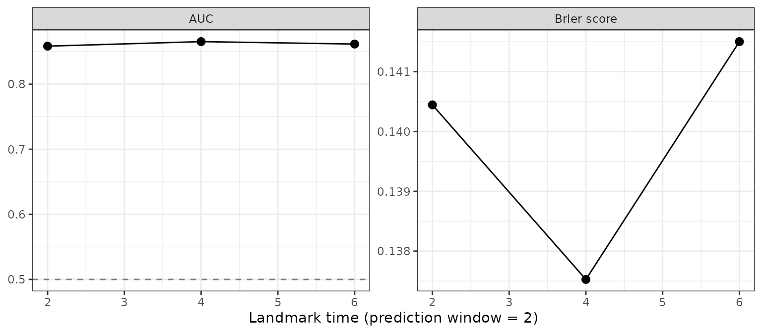

Time-dependent AUC and Brier score at landmark times 2, 4 and 6, model-based.

interval_method = "ipcw" uses only the subjects whose status is certain, reweighted, and does not rely on the model. In simulations with visits every 1–3 years, though, only about 5 of 60 cases had a certain status. The IPCW Brier score came out at about 0.03 instead of the true 0.13, and the IPCW AUC was about three times as variable. The model-based measures stayed within about 0.003 of the truth, even with a misspecified survival sub-model. Because the model grades itself, a miscalibrated model’s Brier score comes out slightly too good, so check calibration separately with calibrationPlot(), which does not use the model.

In calibrationPlot(), each risk group’s observed risk is estimated without the model. A Turnbull-type nonparametric estimate is computed from the intervals and left-truncated at each subject’s last visit, so it targets the same quantity predictRisk() predicts:

calibrationPlot(evaluation, fit$long_fit_all, fit$survival_fit_all,
                prediction_time = c(2, 4), horizon = 2, time_variable = "year",
                survival_variable_all = NULL, survival_trans_function = NULL,
                n_groups = 4, bandcount1 = 20, bandcount2 = 40)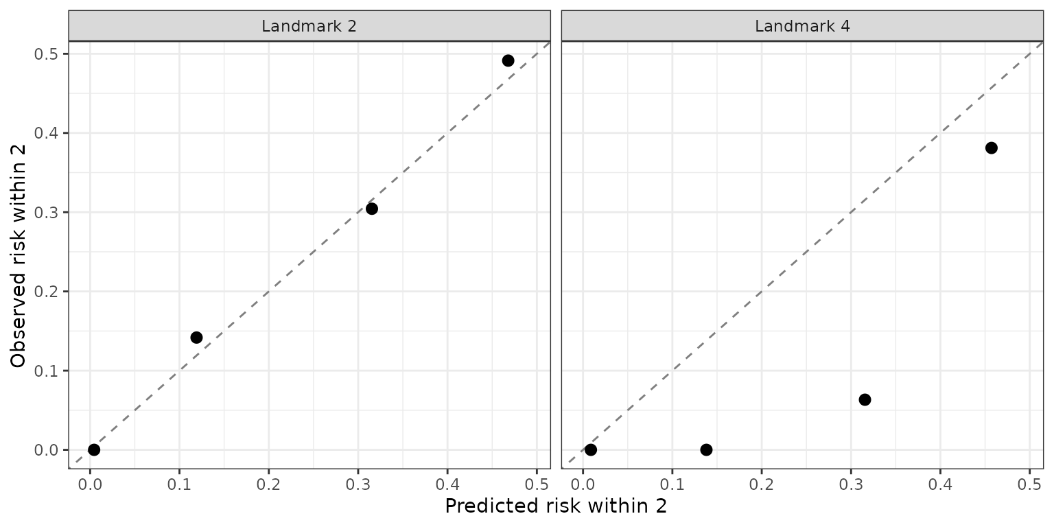

Calibration plot: mean predicted risk against the nonparametric observed risk in four risk groups, at landmarks 2 and 4.

In simulations with visits every 1–3 years and a 2-year window, this observed risk was unbiased for every risk group. It also exposed a deliberately miscalibrated model, where an observed risk computed from the model’s own posterior followed the miscalibrated predictions instead. But with event times known only up to their intervals it is noisy: with groups of about 60 subjects it was off by 0.08–0.16 on average, so a group can sit well off the diagonal by chance, as at landmark 4 here. It also needs the prediction window to be at least about as long as the gaps between visits. With visits every 2–6 years and a 2-year window, the window usually lies inside a subject’s interval, where the timing is not identified, and the observed risk of the higher-risk groups came out up to 0.27 too high. As everywhere in BJM, evaluating on the fitting data gives an optimistic (apparent) performance. Use held-out data when you can.

Assumptions and limitations

Detection at visits. The event is detected at the first visit after it happens, and the visit schedule does not depend on the patient’s risk beyond the observed data (non-informative inspection).
Biomarker visits are inspection visits. The last visit $V$ used in prediction is the last biomarker measurement up to the prediction time.
Before the first visit. The baseline hazard is extrapolated there, so the share of events before the first visit (reported by print()) indicates how much the results lean on it.
Stochastic EM. Each iteration uses one draw of the event times. In an extreme design (visits every 2–6 years), this left a bias of about 2% of the effect. The pooled standard errors treat the model parameters as fixed, so they can be slightly too small.
Experimental. The interface may change. The simulations behind the numbers in this article are kept in a separate folder, next to the package source.

References

Turnbull, B. W. (1976). The empirical distribution function with arbitrarily grouped, censored and truncated data. Journal of the Royal Statistical Society, Series B, 38, 290–295.
Hudgens, M. G., Satten, G. A., & Longini, I. M. (2001). Nonparametric maximum likelihood estimation for competing risks survival data subject to interval censoring and truncation. Biometrics, 57, 74–80.
Royston, P., & Parmar, M. K. B. (2002). Flexible parametric proportional-hazards and proportional-odds models for censored survival data. Statistics in Medicine, 21, 2175–2197.
Yang, Z., Rizopoulos, D., Newcomb, L. F., & Erler, N. S. (2026). Time-dependent predictive accuracy metrics in the context of interval censoring and competing risks. Biometrical Journal, 68, e70108.