Plot predictive performance across landmark times

Evaluates how well the backward joint model's dynamic risk predictions discriminate and are calibrated, at each of several landmark times. For each landmark s in prediction_time, every subject in data_predict_all still event-free at s gets a predicted risk from predictRisk, using only their longitudinal history up to s, of an event in (s, s + horizon]; this is compared with what actually happened, by

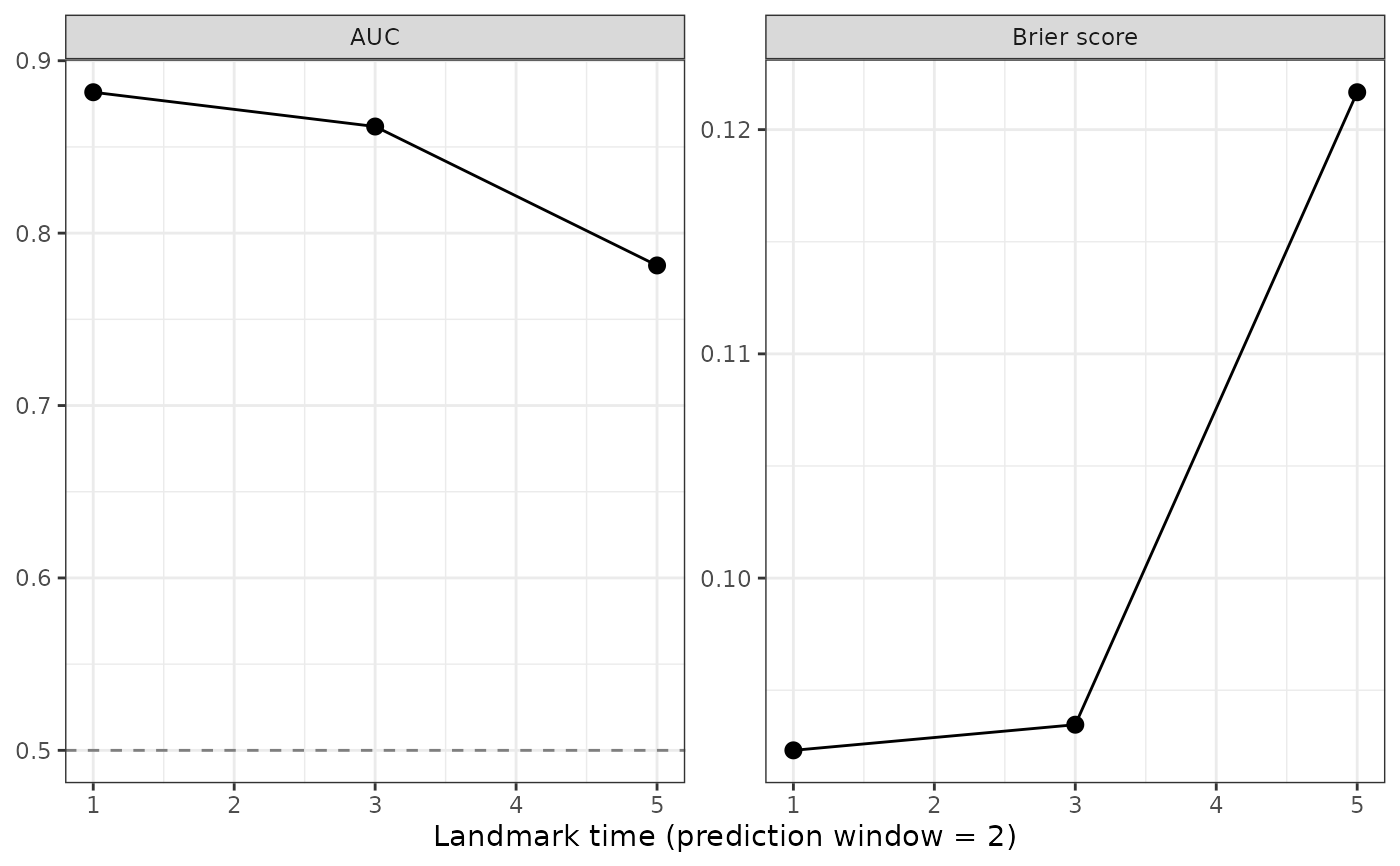
AUC: the time-dependent (cumulative/dynamic) area under the ROC curve: the probability that a subject with an event in the window has a higher predicted risk than one still event-free at s + horizon. 0.5 is no better than chance, 1 is perfect.
Brier score: the mean squared difference between the predicted risk and the observed event indicator in the window. Lower is better.

Subjects censored within the window are handled by inverse probability of censoring weighting (IPCW), with the censoring distribution among the subjects at risk at s estimated by Kaplan–Meier. With competing risks, both measures are computed separately for each event type: the cases are the subjects with that event type in the window, and for the Brier score a subject with the other event type in the window counts as not having the event.

Evaluating on the data the sub-models were fit on gives an optimistic (apparent) performance; pass held-out validation data in data_predict_all when available.

Usage

performancePlot(
  data_predict_all,
  long_fit_all,
  survival_fit_all,
  prediction_time,
  horizon,
  time_variable,
  survival_variable_all,
  survival_trans_function,
  bandcount1 = "auto",
  bandcount2 = "auto",
  interval_method = c("model", "ipcw")
)

Arguments

data_predict_all: The evaluation data, in the same format as for predictRisk: a list of long-format data.frames, one per longitudinal outcome (or a single data.frame used for all). Unlike for predictRisk(), it must also contain each subject's observed outcome: the survival time and status variables of survival_fit_all's Cox formula and, with competing risks, the event type variable of its form_conditional_cr. The outcome is taken from the first data frame and is hidden from predictRisk().
long_fit_all: A longitudinalSub.BJM object from longitudinalSub.
survival_fit_all: A survivalSub.BJM object from survivalSub.
prediction_time: A vector of landmark times.
horizon: The prediction horizon (a single positive number): the window after each landmark in which events are counted.
time_variable: The name of the time variable in the linear mixed models.
survival_variable_all, survival_trans_function: As for predictRisk.
bandcount1, bandcount2: As for predictRisk; passed to it at each landmark.
interval_method: Only for an interval-censored survival_fit_all: "model" (default) or "ipcw"; see Description. For an interval-censored fit, data_predict_all must contain the interval columns of form_marginal_surv (and the event type) instead of a survival time and status.

Value

A ggplot object with one panel per measure, the landmark time on the horizontal axis. Its data element is a data.frame with one row per landmark, measure (and event type), and columns landmark, measure, cause, value, n_at_risk (subjects predicted) and n_cases (events of that type observed in the window).

Interval-censored fits (experimental)

The event is then only known to lie between the last negative visit \(L\) and the visit \(R\) that detected it. A subject is at risk at s when followed up past s without a detected event, and the predicted risk is that of predictRisk() (conditional on being event-free at the last visit). Following Yang, Rizopoulos, Newcomb and Erler (2026, Biometrical Journal 68:e70108), interval_method chooses how subjects whose interval straddles s or s + horizon are handled:

"model" (default): every subject at risk counts, as a case or a control with the probability the fitted model gives their event time given their observed interval. The model only splits the interval observed for each subject, so in our simulations (visits every 1–3 years, 2-year window) both measures were within about 0.003 of their true values, also with a survival sub-model that left out a covariate. The model does grade itself, though: for a deliberately miscalibrated model the Brier score came out slightly too good (by about 0.003), so judge calibration with calibrationPlot, which does not use the model.
"ipcw": only subjects whose status is certain are used – cases detected inside the window after a negative visit at or after s, controls with a negative visit at or after s + horizon – weighted by the inverse Kaplan–Meier probability of still being followed up. It does not use the model, but these weights do not account for how likely the status of a subject is to be certain, which depends on the visit schedule: in the same simulations only about 5 of 60 cases were certain, the Brier score came out at about 0.03 instead of 0.13, and the AUC was about 0.01 too high with three times the error of "model". With visits every 3–9 months the Brier score was still about 25% too low. Use it as a model-free check of the AUC.

Examples

# \donttest{
data(pbc3)
survival_fit_all <- survivalSub(pbc3[!duplicated(pbc3$id), ],
                                Surv(years, status3) ~ age + sex, NULL)
long_sub_fixed <- list("long1" = serBilir ~ year + age + sex + years)
long_sub_random <- list("long1" = ~ year | id)
long_fit_all <- longitudinalSub(list(pbc3[pbc3$status3 == 1, ]),
                                long_sub_fixed, long_sub_random)
trans <- survivalTrans(c(1, 3, 5, 7))

# apparent performance on the fitting data, 2-year window
performancePlot(pbc3, long_fit_all, survival_fit_all,
  prediction_time = c(1, 3, 5), horizon = 2, time_variable = "year",
  trans$survival_variable_all, trans$survival_trans_function)

# }