Plot simulated futures

Plots the draws of simulateTrajectory, pooling every draw of the patients chosen by id (all of them by default: one patient's draws picture that patient's predictive distribution, one draw each of a synthetic cohort pictures the cohort):

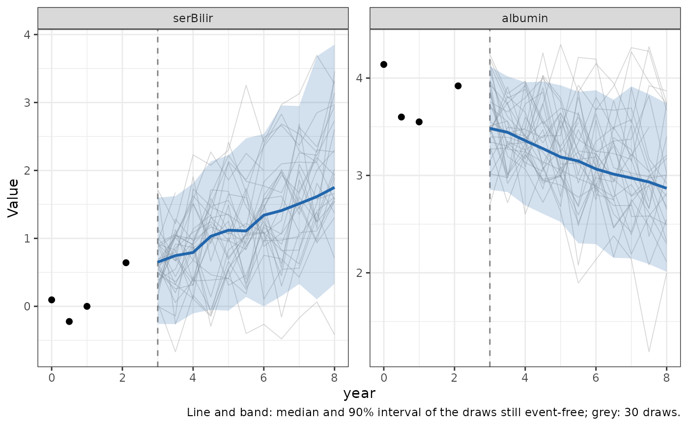
"trajectory"

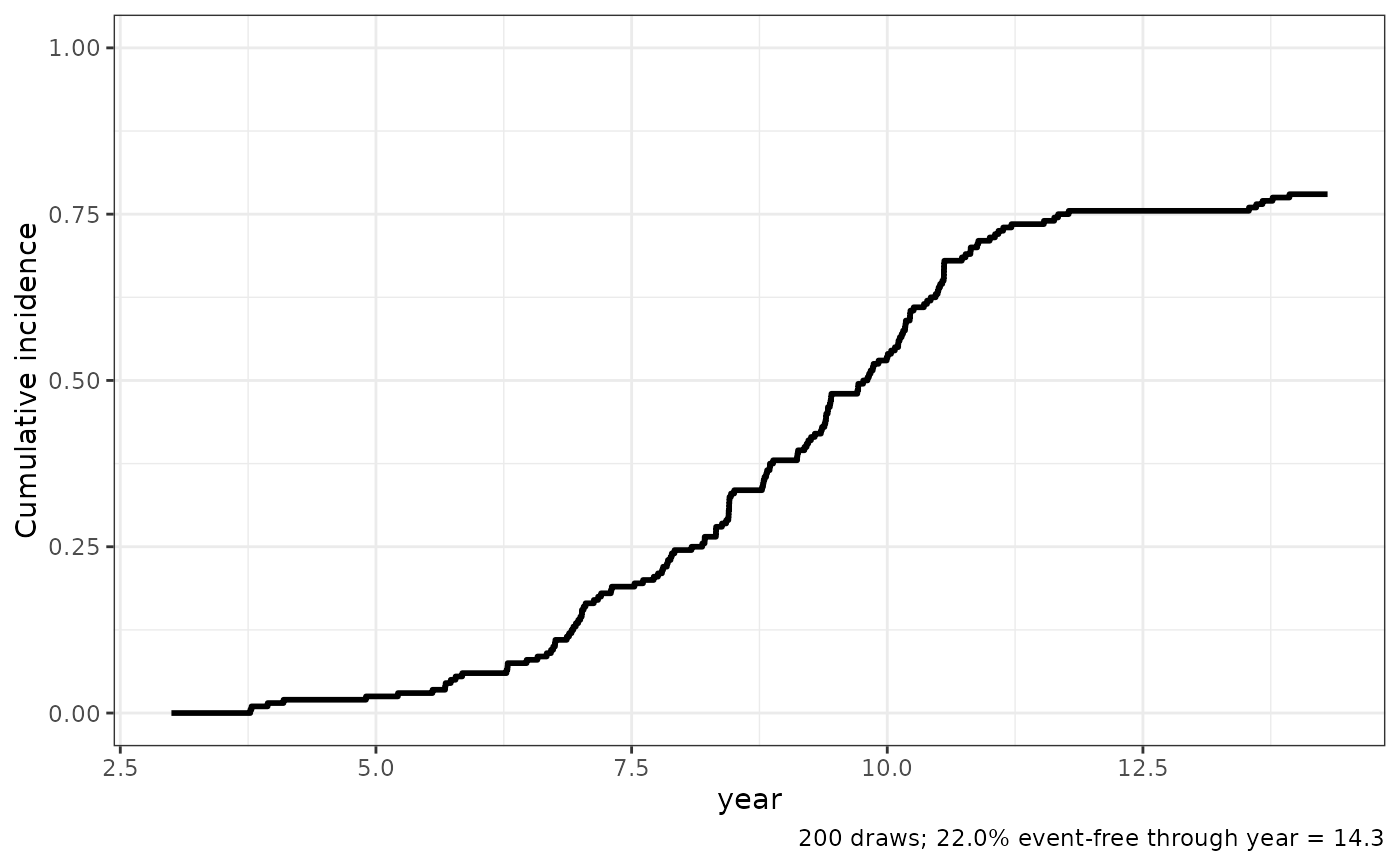
One panel per biomarker. For a continuous biomarker, n_paths of the simulated trajectories as thin lines, with the median and the central level interval of the draws at each time, and the measurements conditioned on as points. For an ordinal biomarker, the share of the draws in each category at each time. With truncate = TRUE in simulateTrajectory() the summaries at a time describe the draws still event-free then.

"event"

The cumulative incidence of the event (of each event type, with competing risks) after prediction_time, computed from the drawn event times.

Usage

# S3 method for class 'simulateTrajectory.BJM'
plot(
  x,
  which = c("trajectory", "event"),
  id = NULL,
  n_paths = 30,
  level = 0.9,
  ...
)

Arguments

x

A simulateTrajectory.BJM object returned by simulateTrajectory.

which

"trajectory" (default) or "event".

id

Patient id(s) whose draws to plot; NULL (default) for all.

n_paths

Number of simulated trajectories drawn as lines (the first ones; the draws are independent, so they are a random sample).

level

Coverage of the interval drawn around the median.

...

Currently unused.

Value

A ggplot object.

Examples

# \donttest{
data(pbc3)
survival_fit_all <- survivalSub(pbc3[!duplicated(pbc3$id), ],
                                Surv(years, status3) ~ age + sex, NULL)
long_fit_all <- longitudinalSub(list(pbc3[pbc3$status3 == 1, ], pbc3[pbc3$status3 == 1, ]),
                                list(serBilir ~ year + age + sex + years,
                                     albumin ~ year + age + sex + years),
                                list(~ year | id, ~ year | id))
history <- pbc3[pbc3$id == 2 & pbc3$year <= 3, ]
sims <- simulateTrajectory(history, long_fit_all, survival_fit_all,
                           prediction_time = 3, times = seq(3, 8, by = 0.5),
                           time_variable = "year", survival_variable_all = list(),
                           survival_trans_function = list(), n_sim = 200, seed = 1)
plot(sims)

plot(sims, which = "event")

# }