Plot a fitted longitudinal sub-model

Diagnostic plots for the per-biomarker mixed models and the shared random-effects covariance of a longitudinalSub fit, one panel per biomarker:

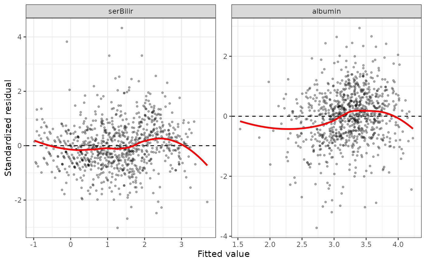
"residuals"

Standardized (Pearson) residuals against fitted values, with a LOESS smoother; a trend or a funnel shape suggests a misspecified mean or non-constant variance.

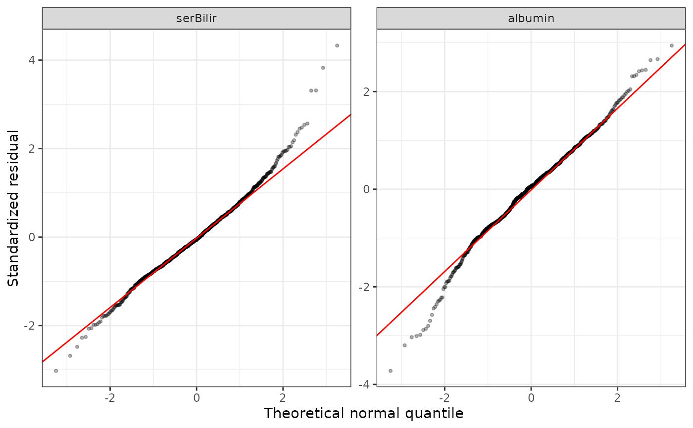
"qq"

Normal Q-Q plot of the standardized residuals.

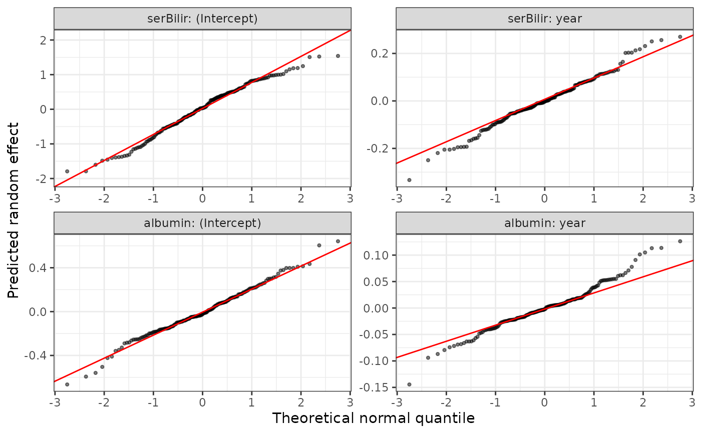
"ranef"

Normal Q-Q plot of each predicted random effect (the model assumes they are normal).

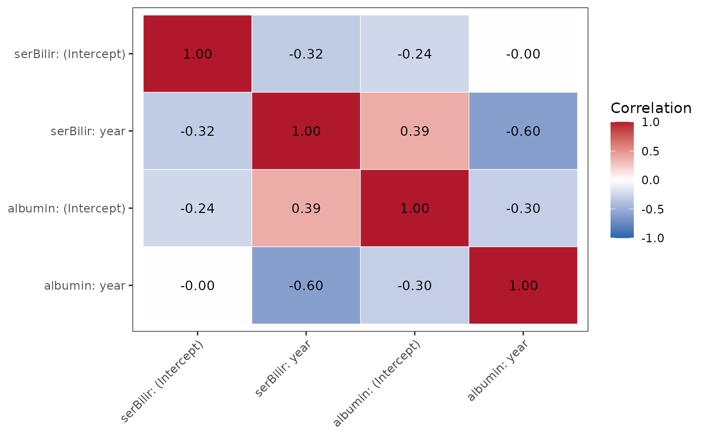
"corr"

Heat map of the correlation matrix of the multivariate random-effects covariance Sigma_fit, i.e. how the subject-level deviations of the different biomarkers move together.

Residual plots are drawn for continuous biomarkers only; an ordinal biomarker (fit by ordinal::clmm()) has no residuals on the response scale and is left out of them with a message.

Usage

# S3 method for class 'longitudinalSub.BJM'
plot(x, which = c("residuals", "qq", "ranef", "corr"), ...)

Arguments

x

A longitudinalSub.BJM object returned by longitudinalSub.

which

Which plot to draw: "residuals" (default), "qq", "ranef" or "corr".

...

Currently unused.

Value

A ggplot object.

Examples

# \donttest{
data(pbc3)
long_sub_fixed <- list("long1" = serBilir ~ year + age + sex + years,
                       "long2" = albumin ~ year + age + sex + years)
long_sub_random <- list("long1" = ~ year | id, "long2" = ~ year | id)
data_fit <- pbc3[pbc3$status3 == 1, ]
long_fit_all <- longitudinalSub(list(data_fit, data_fit), long_sub_fixed, long_sub_random)

plot(long_fit_all)

plot(long_fit_all, which = "qq")

plot(long_fit_all, which = "ranef")

plot(long_fit_all, which = "corr")

# }