Plot risk and future biomarker predictions across a horizon sweep

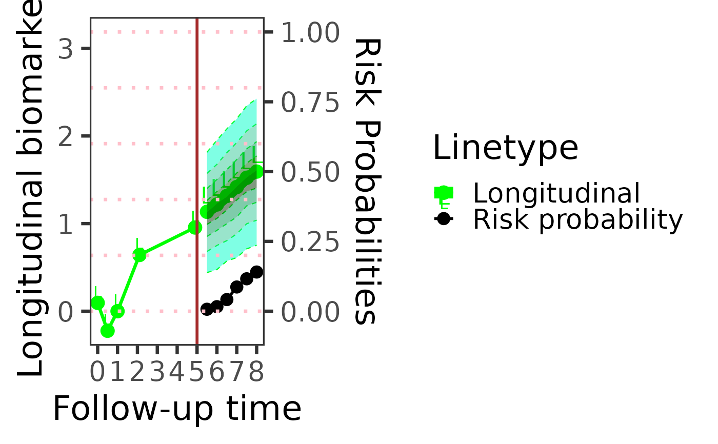
Fixes the landmark time at prediction_time and sweeps forward over a range of prediction horizons, calling predictRisk (and, when bio_pred is supplied, predictLongitudinal) at each horizon to trace out how predicted event risk (and, optionally, the predicted density/point-forecast of biomarker bio_pred) evolves the further out the prediction window extends from a single fixed landmark. This contrasts with riskPlot, which instead fixes the horizon and sweeps over a set of landmark times.

Usage

predictPlot(
  data_predict_all_one,
  long_fit_all,
  survival_fit_all,
  prediction_time = 4,
  horizon = seq(0, 3, 0.5),
  time_variable,
  survival_variable_all,
  survival_trans_function,
  bandcount1 = "auto",
  bandcount2 = "auto",
  bandcount3 = "auto",
  bio_his = 1,
  bio_pred = 1,
  density = 1,
  n_cores = 1
)

Arguments

data_predict_all_one

This involves a collection of data.frame one object for dynamic prediction and making plots, each corresponding to a distinct longitudinal outcome. These data frames should contain the variables specified in long_sub_fixed and long_sub_random. Utilizing a list structure allows for the incorporation of multiple longitudinal outcomes, each potentially following different measurement protocols. In instances where all longitudinal outcomes are recorded at identical time points across patients, a singular data.frame object may be used in a list. Alternatively, a single bare data.frame (not wrapped in a list) may be supplied directly; it is then reused for every longitudinal outcome. It is presumed that each data frame is structured in a long format.

long_fit_all

Outputs from the model fitting process using the nlme package, encompassing the results and parameters obtained from the analysis.

survival_fit_all

Results and parameters generated from the model fitting procedure, utilizing the coxph function. These outputs include the comprehensive findings and variables derived from the analysis.

prediction_time

Time used to make the prediction.

horizon

Prediction horizon.

time_variable

The name of time variable in linear mixed model.

survival_variable_all

The name of the transformed time-to-event outcomes variable.

survival_trans_function

The transformation function used for time-to-event outcomes, in the order of survival_variable_all.

bandcount1

The number of grid points spanning the prediction window, from prediction_time to prediction_time + horizon. Larger values give a more accurate but slower estimate. Defaults to "auto", which resolves it once, before looping over horizon (using the largest requested horizon as a representative probe), by doubling from a built-in starting value until the predicted risk stabilizes; see predictRisk's bandcount1 for details of that search. The resolved value is then reused, fixed, for every point in horizon – it is not re-searched on every iteration.

bandcount2

The number of grid points used to approximate integrating out to infinity when normalizing the predicted risk/density. A wider follow-up range needs a larger bandcount2 to keep the grid spacing comparable. Defaults to "auto"; resolved the same way as bandcount1 (jointly with it, when both are "auto").

bandcount3

The number of points in the candidate-biomarker-value grid used to build the predicted density curve; controls the resolution of the density, not a time integral. Defaults to "auto"; resolved the same way, but only when bio_pred is non-NULL (it is unused otherwise).

Pass explicit numbers instead of "auto" for full manual control, or use checkBandcountConvergence() (applied to predictRisk()/ predictLongitudinal() directly) to inspect the convergence behavior yourself. See also vignette("BJM-intro", package = "BJM") for further guidance on choosing bandcount1/bandcount2/ bandcount3.

bio_his

Which biomarker history will be plotted

bio_pred

Indicator, predict future biomarker or not, if NULL do not predict

density

Indicator, plot future biomarker density or not, if NULL do not plot

n_cores

Number of CPU cores to use for computing the prediction at each point in horizon. Each point is computed independently, so this loop can be dispatched across cores. Defaults to 1 (serial execution; identical behavior/output to versions of this function without this argument). Values greater than 1 use parallel::mclapply(), which relies on forking and is therefore only actually parallel on Unix-like systems (Linux, macOS); on Windows, mclapply() silently runs the iterations serially regardless of n_cores (a limitation of R's fork-based parallelism, not of this package). Parallel execution produces exactly the same numeric result as serial execution – only the order in which iterations are computed (not the order results are assembled in) changes.

Value

Plot of risk and future biomarker with density using dynamic prediction.

Examples

# \donttest{
data(pbc3)

data_survival_fitting =  pbc3[!duplicated(pbc3$id), ]

form_marginal_surv = Surv(years, status3) ~ age + sex
form_conditional_cr = NULL

survival_fit_all = survivalSub(data_survival_fitting, form_marginal_surv, 
                               form_conditional_cr)

long_sub_fixed = list(
  "long1" = serBilir ~ year + age + sex +  (years) + (years) * year,  
  "long2" = prothrombin ~ year + age + sex + (years) + (years) * year,  
  "long3" = albumin ~ year + age + age * year + sex + (years) + (years) * year,  
  "long4" = alkaline ~ year + age + sex + (years) + (years) * year, 
  "long5" = SGOT ~ year + age + sex + (years) + (years) * year, 
  "long6" = platelets ~ year + age + sex + (years)  + (years) * year)

long_sub_random =list(
  "long1" =  ~ year| id,   
  "long2" =  ~ year| id,    
  "long3" =  ~ year| id,    
  "long4" =  ~ year| id,    
  "long5" =  ~ year| id,    
  "long6" =  ~ year| id)

survival_variable_all = list(
  "Tyears1",  "Tyears2", "Tyears3", "Tyears4"
)

survival_trans_function = list(
  fun1 = function(x){abs(x - 1)}, 
  fun2 = function(x){abs(x - 3)}, 
  fun3 = function(x){abs(x - 5)}, 
  fun4 = function(x){abs(x - 7)}
)

# Complete case analysis
data_fit_all = list()
for(i in seq_len(length(long_sub_fixed))){
  data_fit_all[[i]] = pbc3[pbc3$status3 == 1, ]
}

# fitting longitudinal submodel
long_fit_all = longitudinalSub(data_fit_all, long_sub_fixed, long_sub_random)

i_PID = 2
data.raw.predict.plot = pbc3[pbc3$id == i_PID, ]
data_predict_all_one = list(data.raw.predict.plot, data.raw.predict.plot, data.raw.predict.plot,
                            data.raw.predict.plot, data.raw.predict.plot, data.raw.predict.plot)

# plot biomarker 1 history,  predict future biomarker

predictPlot(data_predict_all_one, long_fit_all, survival_fit_all,
            prediction_time = 5, bio_his = 1, bio_pred = 1,
            horizon = seq(0.5, 3.0, 0.5), time_variable = "year",
            survival_variable_all, survival_trans_function,
           bandcount1 = 10, bandcount2 = 10, bandcount3 = 200)

       
# }