Plot predicted risk across a sweep of landmark times

Fixes the prediction horizon and sweeps backward/forward over a set of landmark times, calling predictRisk at each landmark in prediction_time to trace out how predicted event risk over that fixed-length window changes as the landmark moves – i.e. as more (or less) of the subject's longitudinal history is used to update their risk. prediction_time may be a vector of landmark times to use directly; a single value, which is expanded to three landmarks (prediction_time, 1.5 * prediction_time, 2 * prediction_time); or NULL, which uses every observed longitudinal measurement time (across subjects, from the first biomarker's data) as a landmark. This contrasts with predictPlot, which instead fixes the landmark and sweeps over a range of horizons. The optional bio_i argument only selects which biomarker's observed trajectory is overlaid on the plot for visual reference – it does not affect the risk computation itself (unlike predictPlot's bio_pred, which drives a biomarker density prediction).

Usage

riskPlot(
  data_predict_all_pre,
  long_fit_all,
  survival_fit_all,
  prediction_time = NULL,
  bio_i = NULL,
  horizon,
  time_variable,
  survival_variable_all,
  survival_trans_function,
  bandcount1 = "auto",
  bandcount2 = "auto",
  n_cores = 1
)

Arguments

data_predict_all_pre

This involves a collection of data.frame objects for dynamic prediction, each corresponding to a distinct longitudinal outcome. These data frames should contain the variables specified in long_sub_fixed and long_sub_random. Utilizing a list structure allows for the incorporation of multiple longitudinal outcomes, each potentially following different measurement protocols. In instances where all longitudinal outcomes are recorded at identical time points across patients, a singular data.frame object may be used in a list. Alternatively, a single bare data.frame (not wrapped in a list) may be supplied directly; it is then reused for every longitudinal outcome. It is presumed that each data frame is structured in a long format.

long_fit_all

Outputs from the model fitting process using the nlme package, encompassing the results and parameters obtained from the analysis.

survival_fit_all

Results and parameters generated from the model fitting procedure, utilizing the coxph function. These outputs include the comprehensive findings and variables derived from the analysis.

prediction_time

The landmark time(s) at which risks are predicted and plotted: NULL (the default) uses every visit time (time_variable) in the patient's data; a single value s uses the three landmarks s, 1.5 * s and 2 * s; a vector uses those times. At each landmark only the history up to it is used.

bio_i

Biomarker whose observed history is drawn alongside the predicted risks (by position in long_fit_all); NULL draws the first one.

horizon

Prediction horizon.

time_variable

The name of time variable in linear mixed model.

survival_variable_all

The name of the transformed time-to-event outcomes variable.

survival_trans_function

The transformation function used for time-to-event outcomes, in the order of survival_variable_all.

bandcount1

The number of grid points spanning the prediction window, from prediction_time to prediction_time + horizon. Larger values give a more accurate but slower estimate. Defaults to "auto", which resolves it once, before looping over the landmark times, (using the first landmark time as a representative probe) by doubling from a built-in starting value until the predicted risk stabilizes; see predictRisk's bandcount1 for details of that search. The resolved value is then reused, fixed, for every landmark time – it is not re-searched on every iteration.

bandcount2

The number of grid points used to approximate integrating out to infinity when normalizing the predicted risk. A wider follow-up range needs a larger bandcount2 to keep the grid spacing comparable. Defaults to "auto"; resolved the same way as bandcount1 (jointly with it, when both are "auto").

Pass explicit numbers instead of "auto" for full manual control, or use checkBandcountConvergence() (applied to predictRisk() directly) to inspect the convergence behavior yourself. See also vignette("BJM-intro", package = "BJM") for further guidance on choosing bandcount1/bandcount2.

n_cores

Number of CPU cores to use for computing the prediction at each landmark time in prediction_time. Each landmark time is computed independently, so this loop can be dispatched across cores. Defaults to 1 (serial execution; identical behavior/output to versions of this function without this argument). Values greater than 1 use parallel::mclapply(), which relies on forking and is therefore only actually parallel on Unix-like systems (Linux, macOS); on Windows, mclapply() silently runs the iterations serially regardless of n_cores (a limitation of R's fork-based parallelism, not of this package). Parallel execution produces exactly the same numeric result as serial execution – only the order in which iterations are computed (not the order results are assembled in) changes.

Value

Plot of risk using dynamic prediction.

Examples

# \donttest{
data(pbc3)
survival_fit_all <- survivalSub(pbc3[!duplicated(pbc3$id), ],
                                Surv(years, status3) ~ age + sex, NULL)
long_fit_all <- longitudinalSub(pbc3[pbc3$status3 == 1, ],
                                list(serBilir ~ year + age + sex + years,
                                     albumin ~ year + age + sex + years),
                                list(~ year | id, ~ year | id))

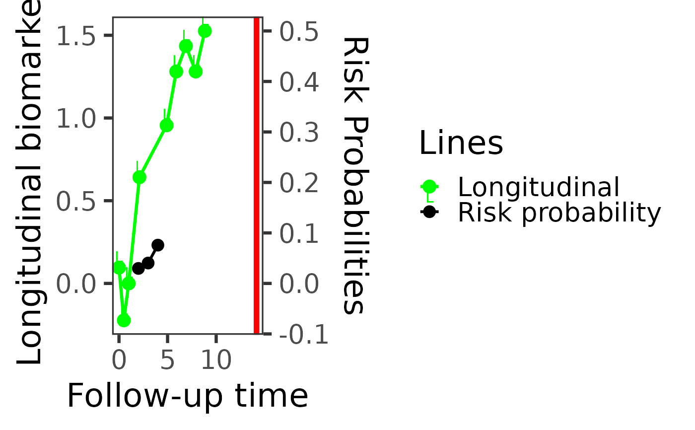
# one patient's whole history; risks within 2 years of landmarks 2, 3, 4
patient <- pbc3[pbc3$id == 2, ]
riskPlot(patient, long_fit_all, survival_fit_all, prediction_time = c(2, 3, 4),
         bio_i = 1, horizon = 2, time_variable = "year",
         survival_variable_all = list(), survival_trans_function = list(),
         bandcount1 = 10, bandcount2 = 20)

# }