Categorical biomarkers

Not every repeated measurement is a number. A symptom can be graded (none, mild, severe), a finding can be present or absent, a disease can be staged. BJM accepts such ordinal biomarkers, including binary ones, next to continuous ones, and uses them for every prediction: the risk of an event, the future category of the biomarker itself, and simulated futures.

Step	Function	With a categorical biomarker
Fit	`longitudinalSub()`	an ordered-factor response is fit as an ordinal biomarker
Predict	`predictRisk()`	the observed categories inform the risk
Predict	`predictLongitudinal()`	the probability of each category at a future time
Plot	`predictPlot()`, `riskPlot()`	the categories on the biomarker axis
Simulate	`simulateTrajectory()`	simulated categories

Fitting an ordinal biomarker needs the ordinal package (in Suggests):

library(BJM)
data(pbc3)
requireNamespace("ordinal", quietly = TRUE)

How BJM models a category

Behind each ordinal measurement, BJM assumes a continuous latent score that follows a linear mixed model, just like a continuous biomarker, and that is cut into the observed categories at estimated thresholds. This is a probit cumulative link mixed model, fit with ordinal::clmm(). A binary biomarker is the special case of two categories and one threshold.

The latent scores and the continuous biomarkers share one joint random-effects distribution (a Gaussian copula). So a patient’s categories tell the model about their continuous biomarkers and the other way round, and both inform the event risk. longitudinalSub() estimates this joint covariance by maximum likelihood, with an EM algorithm that integrates over the ordinal random effects by adaptive Gauss–Hermite quadrature; with more than four ordinal random effects in all it switches to a stochastic approximation EM.

The data

edema in pbc3 is recorded at every visit in three ordered categories: no edema, edema without diuretics or resolved by them, and edema despite diuretics. We give the categories short names and make the column an ordered factor, which is how BJM recognizes an ordinal biomarker. The order of the levels is the order of the categories.

pbc3$edema <- factor(pbc3$edema, labels = c("none", "controlled", "persistent"),
                     ordered = TRUE)
table(pbc3$edema)
#> 
#>       none controlled persistent 
#>       1401        379        165

Edema changes during follow-up for many patients:

changes <- tapply(as.integer(pbc3$edema), pbc3$id, function(x) length(unique(x)) > 1)
sum(changes)
#> [1] 146

Fitting

The survival sub-model is the usual one, here with competing risks (death and transplantation, see the Competing risks article):

survival_fit <- survivalSub(pbc3[!duplicated(pbc3$id), ],
                            Surv(years, status3) ~ age + sex,
                            status4 ~ years + age + sex)

The ordinal biomarker gets a formula and random effects like any other. Because edema is an ordered factor, longitudinalSub() fits it as ordinal and serBilir as continuous; biomarker_type = c("continuous", "ordinal") would say the same explicitly. The model has no intercept: the thresholds take its place.

long_fit <- longitudinalSub(
  pbc3[pbc3$status3 == 1, ],
  list(serBilir = serBilir ~ year + age + sex + years + years:year,
       edema    = edema ~ year + age + years + years:year),
  list(serBilir = ~ year | id, edema = ~ 1 | id)
)
long_fit$biomarker_type
#> [1] "continuous" "ordinal"

(ordinal::clmm() may warn about a non-finite log-likelihood at an intermediate iteration of its optimizer; this one does, and the warning is hidden above. It is harmless when the fit converges, as it does here: the largest gradient at the optimum is below 0.01.)

long_fit
#> 
#> Call:
#> longitudinalSub(M = 2 longitudinal outcomes)
#> 
#> =================================================================
#>  Longitudinal Sub-model(s)
#> -----------------------------------------------------------------
#>  [1] serBilir (continuous)
#>  Formula: serBilir ~ year + age + sex + years + years:year
#> 
#>                 Value        SE      t  p-value    
#> (Intercept)  2.424554  0.384604  6.304 5.13e-10 ***
#> year         0.442242  0.042957 10.295  < 2e-16 ***
#> age         -0.011675  0.005785 -2.018   0.0439 *  
#> sex          0.078449  0.167140  0.469   0.6390    
#> years       -0.204130  0.021557 -9.469  < 2e-16 ***
#> year:years  -0.027852  0.006112 -4.557 6.12e-06 ***
#> ---
#> Signif. codes:  0 '***' 0.001 '**' 0.01 '*' 0.05 '.' 0.1 ' ' 1
#> 
#>   Residual std. error (sigma): 0.4186
#>   n (subjects) = 169,  N (observations) = 872
#>   Log-likelihood: -772.87
#>   AIC: 1565.74,  BIC: 1613.45
#> 
#> -----------------------------------------------------------------
#>  [2] edema (ordinal)
#>  Formula: edema ~ year + age + years + years:year
#> 
#>               Value       SE      z  p-value    
#> year        0.68832  0.09263  7.431 1.08e-13 ***
#> age         0.03636  0.01152  3.155  0.00160 ** 
#> years      -0.31621  0.04716 -6.705 2.01e-11 ***
#> year:years -0.03090  0.01030 -2.999  0.00271 ** 
#> ---
#> Signif. codes:  0 '***' 0.001 '**' 0.01 '*' 0.05 '.' 0.1 ' ' 1
#> 
#>   Cumulative thresholds (probit link):
#>       none|controlled controlled|persistent 
#>                1.5776                3.1078 
#> 
#>   n (subjects) = 169,  N (observations) = 872
#>   Log-likelihood: -606.53
#>   AIC: 1227.06,  BIC: 1260.45
#> 
#> =================================================================
#>  Multivariate Random-Effects Covariance Matrix (D)
#> -----------------------------------------------------------------
#>               (Intercept)_1  year_1 (Intercept)_2
#> (Intercept)_1        0.6005 -0.0205        0.1795
#> year_1              -0.0205  0.0180        0.0086
#> (Intercept)_2        0.1795  0.0086        1.8783
#> =================================================================

For edema, the printed fit shows the coefficients of the latent score and the two thresholds between the three categories. Edema becomes more likely over follow-up (year) and the closer a patient is to the event (years). The last table is the joint covariance of the random effects: the edema intercept is positively correlated with the bilirubin intercept, so patients with more edema tend to have higher bilirubin.

A binary biomarker

A two-level factor is a binary biomarker, fit the same way. Here ascites (No/Yes) is added as a third biomarker:

long_fit_3 <- longitudinalSub(
  pbc3[pbc3$status3 == 1, ],
  list(serBilir ~ year + age + sex + years + years:year,
       edema ~ year + age + years + years:year,
       ascites ~ year + years),
  list(~ year | id, ~ 1 | id, ~ 1 | id)
)
long_fit_3$biomarker_type
#> [1] "continuous" "ordinal"    "ordinal"
round(cov2cor(long_fit_3$Sigma_fit), 2)
#>               (Intercept)_1 year_1 (Intercept)_2 (Intercept)_3
#> (Intercept)_1          1.00  -0.19          0.18          0.17
#> year_1                -0.19   1.00          0.07          0.31
#> (Intercept)_2          0.18   0.07          1.00          0.85
#> (Intercept)_3          0.17   0.31          0.85          1.00

Edema and ascites are strongly correlated (0.85): both reflect fluid retention.

Predicting the event risk with `predictRisk()`

Patient 2 had no edema at the first four visits, and controlled edema at the visit just before year 5:

patient <- pbc3[pbc3$id == 2 & pbc3$year <= 5, ]
patient$years <- NA
patient$status4 <- NA
patient[, c("year", "serBilir", "edema")]
#>        year    serBilir      edema
#> 3 0.0000000  0.09531018       none
#> 4 0.4983025 -0.22314355       none
#> 5 0.9993429  0.00000000       none
#> 6 2.1027270  0.64185389       none
#> 7 4.9008871  0.95551145 controlled

predictRisk() is called as usual. With an ordinal biomarker, each patient’s likelihood includes the probability of their observed categories. With one ordinal random effect, as here, BJM computes it by numerical integration over that random effect, so the results are exact and the same on every run.

risk <- predictRisk(list(patient, patient), long_fit, survival_fit,
                    prediction_time = 5, horizon = 3, time_variable = "year",
                    survival_variable_all = list(), survival_trans_function = list())
risk
#> 
#> =================================================================
#>  Dynamic Prediction - Event Risk
#> -----------------------------------------------------------------
#>   Competing risks   : Yes
#>   Subjects          : 1
#> -----------------------------------------------------------------
#> 
#>  Subject Cause 1 Risk Cause 2 Risk Total Risk
#>        2       0.4258       0.0182      0.444
#> 
#> =================================================================

The categories matter. Had the last visit shown no edema, the predicted risk of death within three years would be about half as large:

no_edema <- patient
no_edema$edema[nrow(no_edema)] <- "none"
risk_no_edema <- predictRisk(list(no_edema, no_edema), long_fit, survival_fit,
                             prediction_time = 5, horizon = 3, time_variable = "year",
                             survival_variable_all = list(), survival_trans_function = list())
c(observed = unname(risk$risk_prob_1), if_no_edema = unname(risk_no_edema$risk_prob_1))
#>    observed if_no_edema 
#>   0.4258237   0.2350548

The categories in the prediction data are matched to those of the fit by their labels, so a character column or a factor with its levels in a different order works too; a category the model was not fit with is an error.

Predicting the future category with `predictLongitudinal()`

For an ordinal biomarker, predictLongitudinal() predicts the probability of each category at prediction_time + horizon, for a patient still event-free then. Here for three patients, one year after year 3:

three <- pbc3[pbc3$id %in% c(2, 4, 5) & pbc3$year <= 3, ]
three$years <- NA
three$status4 <- NA
edema_pred <- predictLongitudinal(bio_i = 2, list(three, three), long_fit, survival_fit,
                                  prediction_time = 3, horizon = 1, time_variable = "year",
                                  survival_variable_all = list(), survival_trans_function = list())
edema_pred
#> 
#> =================================================================
#>  Dynamic Prediction - Future Biomarker
#> -----------------------------------------------------------------
#>   Categories        : 3
#>   Subjects          : 3
#> -----------------------------------------------------------------
#> 
#>  Subject P(none) P(controlled) P(persistent) Most.likely
#>        2  0.7851        0.1837        0.0313        none
#>        4  0.0173        0.1992        0.7835  persistent
#>        5  0.0947        0.4054        0.4999  persistent
#> 
#>   P(.) = predicted probability of each category; Most.likely = its mode.
#> 
#> =================================================================

In the returned object, Y_density holds the probabilities (one column per patient), Y_all the category codes 1, 2, 3 with their labels in the "category_labels" attribute, and Y_predict the code of the most likely category. plot() draws the probabilities:

plot(edema_pred)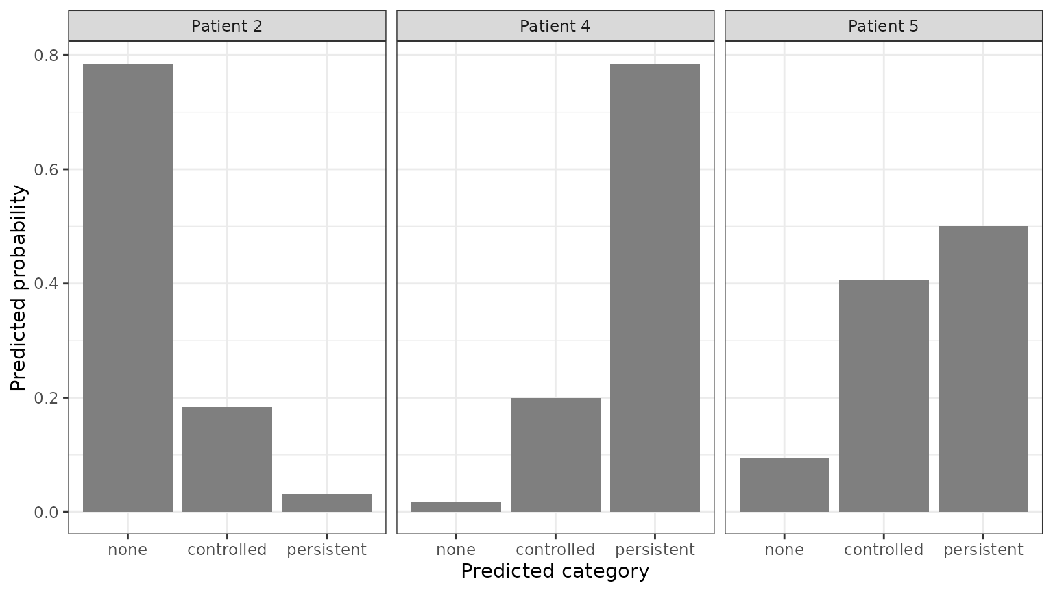

Bar charts of the predicted probabilities of no, controlled and persistent edema one year after year 3, one panel per patient: patient 2 most likely has none (about 0.79), patient 4 persistent (about 0.78), and patient 5 is split between controlled (0.41) and persistent (0.50).

With bio_i = NULL every biomarker is predicted in one call, continuous and ordinal alike:

both <- predictLongitudinal(bio_i = NULL, list(three, three), long_fit, survival_fit,
                            prediction_time = 3, horizon = 1, time_variable = "year",
                            survival_variable_all = list(), survival_trans_function = list())
names(both)
#> [1] "serBilir" "edema"
both$edema$Y_density
#>               2          4          5
#> [1,] 0.78507044 0.01728125 0.09469616
#> [2,] 0.18366320 0.19922645 0.40543314
#> [3,] 0.03126594 0.78349229 0.49987070

Plotting a patient’s predictions

predictPlot() shows the history of one biomarker, chosen with bio_his, with its categories on the vertical axis, the risks of the two event types, and the predicted category probabilities as the horizon grows, as circles whose size is the probability:

predictPlot(list(patient, patient), long_fit, survival_fit,
            prediction_time = 5, horizon = seq(0, 3, 0.5), time_variable = "year",
            survival_variable_all = list(), survival_trans_function = list(),
            bio_his = 2, bio_pred = 2)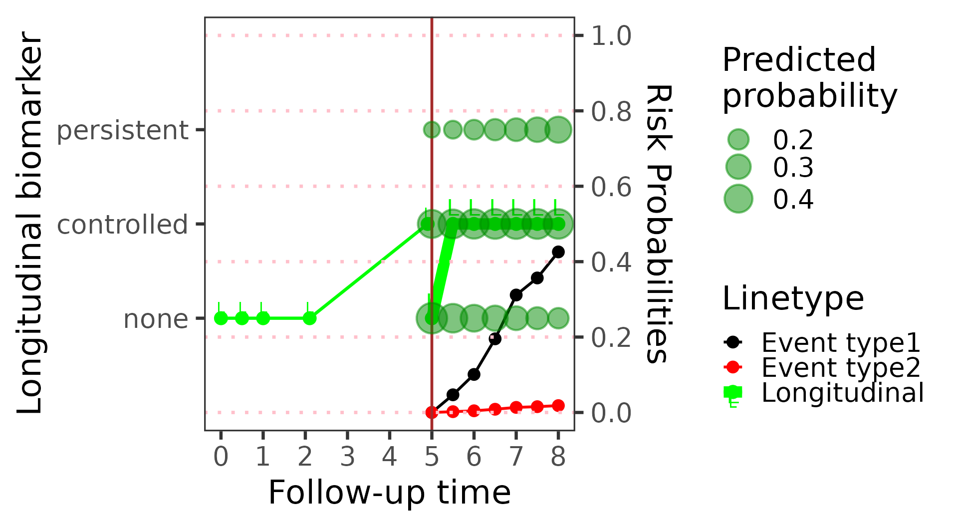

Prediction plot for patient 2 at year 5 with edema on the vertical axis: no edema at the first four visits and controlled edema just before year 5; after year 5, circles show the predicted probabilities of each category up to year 8, with controlled and none most likely and persistent growing; the risk of death rises to about 0.43 by year 8 and that of transplantation stays near 0.

riskPlot() moves the landmark instead; the risk of death rises when the edema appears:

riskPlot(list(patient, patient), long_fit, survival_fit,
         prediction_time = c(1, 2, 3, 4, 5), bio_i = 2, horizon = 1, time_variable = "year",
         survival_variable_all = list(), survival_trans_function = list())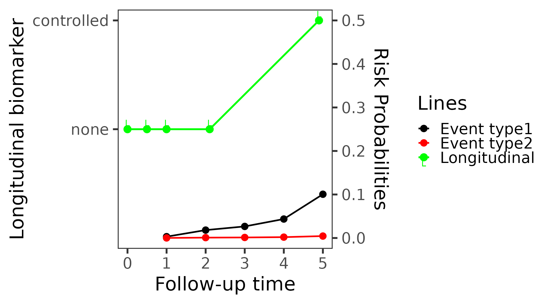

Patient 2's edema history, none until year 2 and controlled just before year 5, with the predicted one-year risks of death and transplantation at landmarks 1 to 5; the risk of death stays below 0.05 until year 4 and rises to about 0.1 at year 5, and transplantation stays near 0.

Simulated futures with `simulateTrajectory()`

Simulated futures draw a latent score for the ordinal biomarker and cut it at the thresholds, so the draws are categories:

sims <- simulateTrajectory(list(patient, patient), long_fit, survival_fit,
                           prediction_time = 5, times = seq(5, 10, 0.5), time_variable = "year",
                           survival_variable_all = list(), survival_trans_function = list(),
                           n_sim = 300, seed = 1)
head(as.data.frame(sims)[, c("sim", "year", "serBilir", "edema")])
#>   sim year  serBilir      edema
#> 1   1  5.0 1.8500962 persistent
#> 2   1  5.5 1.0121664 persistent
#> 3   1  6.0 0.8941778 persistent
#> 4   1  6.5 2.0523262       none
#> 5   1  7.0 1.5222769 persistent
#> 6   1  7.5        NA       <NA>

plot() shows, at each time, the share of the draws still event-free in each category:

plot(sims)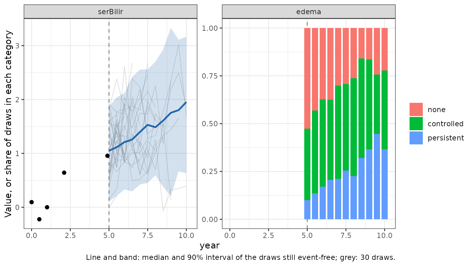

Simulated futures of patient 2 from year 5 to 10 in two panels: for bilirubin, the observed values as points with simulated trajectories and a median rising from about 1 to 2; for edema, stacked bars of the share of draws in each category, with no edema falling from about half to about a quarter and persistent edema rising from about 0.1 to about 0.45.

Things to watch for

Make the response an ordered factor, with its levels in the order of the categories, or pass biomarker_type. A numeric column is fit as a continuous biomarker.
Formulas. An ordinal biomarker’s design matrix is built from the data at hand, not from the training data, so terms whose values depend on the other rows – orthogonal poly(), splines::ns()/bs(), factor() – give wrong predictions; longitudinalSub() warns about them. Use poly(..., raw = TRUE), I(x^2) or log() instead (see the Nonlinear terms article).
Two or more ordinal random effects. The probability of a patient’s observed categories is then computed by Monte Carlo (mvtnorm::pmvnorm()) instead of numerical integration, with an error in about the fourth significant digit (each patient’s draws use a fixed seed, so the results are still the same on every run), and predictions are several times slower. n_cores in predictRisk() and predictLongitudinal() spreads the patients over several cores (on Linux and macOS).
Speed. That probability is needed at every point of the integration grid, so a prediction with an ordinal biomarker takes longer than with continuous ones only. Predicting a continuous biomarker’s future value in a model with an ordinal one is the slowest case; fixed bandcount2/bandcount3 values (checked with checkBandcountConvergence()) are faster than the automatic ones.
Random effects. Up to four ordinal random effects in all (e.g. two ordinal biomarkers with a random intercept and slope each) are integrated by quadrature; beyond that, the stochastic approximation EM is less precise (random-effects variances off by about 5% in simulations).