Competing risks

Often a patient can have one of several events, and having one rules out the others. In pbc3, a patient with primary biliary cirrhosis can die or receive a liver transplant; once transplanted, the patient can no longer die of the untreated disease. These are competing risks. Treating the competing event as censoring overstates the risk of the event of interest, so BJM models both event types together and predicts the risk of each.

This article covers every step of an analysis with two competing event types:

Step	Function	With competing risks
Look at the data	`cifPlot()`	cumulative incidence of each event type
Fit	`survivalSub()`	adds a model for the event type
Fit	`longitudinalSub()`	unchanged; the biomarkers may depend on the event type
Predict	`predictRisk()`	the risk of each event type
Predict	`predictLongitudinal()`	the biomarker’s future value, given no event of either type
Predict	`predictPlot()`, `riskPlot()`	both risks in one plot
Simulate	`simulateTrajectory()`	the event time and type of each simulated future
Evaluate	`performancePlot()`, `calibrationPlot()`	AUC, Brier score and calibration per event type

library(BJM)
data(pbc3)

The data

pbc3 has one row per visit. Three columns describe the outcome, and they are constant within a patient:

years: time from registration to the event or to censoring;
status3: 1 if the patient had an event (death or transplant), 0 if censored;
status4: the event type, 0 for death and 1 for transplantation, and NA for a censored patient.

(status5 codes the same information in one column, 0 censored, 1 death and 2 transplant, which is the form cifPlot() takes.)

first <- pbc3[!duplicated(pbc3$id), ]
table(event = first$status3, type = first$status4, useNA = "ifany")
#>      type
#> event   0   1 <NA>
#>     0   0   0  143
#>     1 140  29    0

Of the 312 patients, 140 died, 29 were transplanted and 143 were censored. The cumulative incidence of each event type, estimated with the Aalen–Johansen estimator, treats the other event correctly rather than as censoring:

cifPlot(pbc3, survival_variable = "years", event_type_variable = "status5",
        event_labels = c("1" = "Death", "2" = "Transplant"))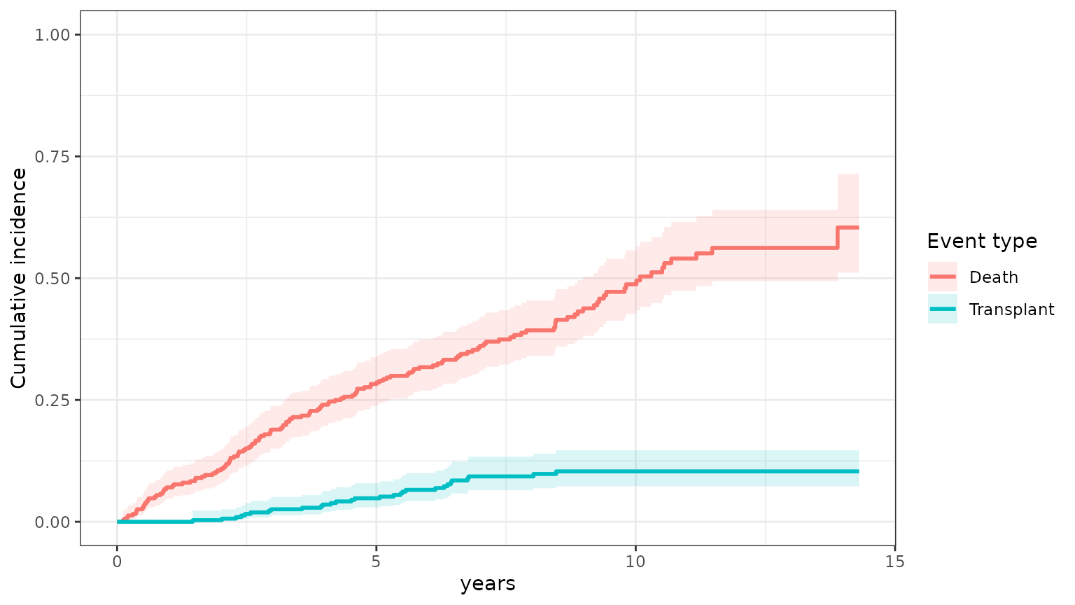

Cumulative incidence curves with 95% confidence bands for death and transplantation over 15 years of follow-up; death reaches about 0.6 while transplantation levels off near 0.1.

Step 1: the survival sub-model

The backward joint model writes the joint distribution of the event time $T$ and the event type $D$ as

$P(T, D) = f(T) \, P(D \mid T),$

a model for when some event happens, and a model for which event it is given when it happens. survivalSub() fits both, from one row per patient:

form_marginal_surv, a Cox model for the time to the first event of either type (status3);
form_conditional_cr, a logistic regression for the event type (status4) among the patients who had an event. It must contain the event time (years), as a plain linear term: this is how the chance of each type can change over time.

survival_fit <- survivalSub(
  first,
  form_marginal_surv = Surv(years, status3) ~ age + sex,
  form_conditional_cr = status4 ~ years + age + sex
)
survival_fit
#> 
#> Call:
#> survivalSub(form_marginal_surv = Surv(years, status3) ~ age + sex,
#>             form_conditional_cr = status4 ~ years + age + sex)
#> 
#> Data Descriptives:
#>   Number of subjects        : 312
#>   Number of events          : 169
#>   Cause-1 events (status4 = 0) : 140
#>   Cause-2 events (status4 = 1) : 29
#> 
#> =================================================================
#>  Marginal Survival Sub-model  [Cox PH]
#> -----------------------------------------------------------------
#>  Formula: Surv(years, status3) ~ age + sex
#> 
#>          Coef exp(Coef)        SE      z p-value   
#> age  0.020411  1.020621  0.007584  2.691 0.00712 **
#> sex -0.497707  0.607923  0.207078 -2.403 0.01624 * 
#> ---
#> Signif. codes:  0 '***' 0.001 '**' 0.01 '*' 0.05 '.' 0.1 ' ' 1
#> 
#>   n = 312,  events = 169
#>   Concordance       = 0.570  (se = 0.0226)
#>   Likelihood ratio  = 14.20  on 2 df,  p = 0.0008263
#>   Wald test         = 15.29  on 2 df,  p = 0.0004776
#>   Score (logrank)   = 15.50  on 2 df,  p = 0.0004299
#> 
#> =================================================================
#>  Conditional Competing-Risks Sub-model  [Logistic GLM]
#> -----------------------------------------------------------------
#>  Formula: status4 ~ years + age + sex
#> 
#>                 Coef       SE      z  p-value    
#> (Intercept)  5.65622  1.70478  3.318 0.000907 ***
#> years       -0.02898  0.08919 -0.325 0.745242    
#> age         -0.15305  0.03076 -4.976  6.5e-07 ***
#> sex          0.02109  0.77150  0.027 0.978192    
#> ---
#> Signif. codes:  0 '***' 0.001 '**' 0.01 '*' 0.05 '.' 0.1 ' ' 1
#> 
#>   Null deviance     : 154.94  on 168 df
#>   Residual deviance : 115.05  on 165 df
#>   AIC : 123.05
#> =================================================================

“Cause 1” is the event type coded 0, death, and “cause 2” the type coded 1, transplantation, the same order the predictions below use. The event-type model’s coefficients are log odds of transplantation against death: older patients are much less likely to be transplanted, while the timing of the event makes little difference (years, p = 0.75).

plot(survival_fit)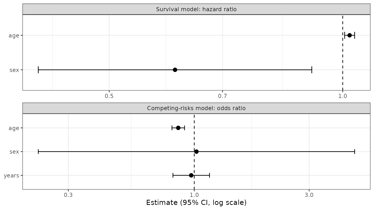

Forest plot in two panels: hazard ratios of the survival model, where age is slightly above 1 and sex is below 1 with a wide interval, and odds ratios of the event-type model for age, sex and event time, all close to 1 except age, slightly below 1.

Without competing risks, leave form_conditional_cr out (or set it to NULL): every prediction below then refers to the single event.

Step 2: the longitudinal sub-models

The biomarker models do not change. As usual, they are fit on the patients with an event, whose event time is known, and contain the event time (years) as a covariate:

long_sub_fixed <- list(
  "serBilir" = serBilir ~ year + age + sex + years + years:year,
  "albumin"  = albumin  ~ year + age + sex + years + years:year
)
long_sub_random <- list("serBilir" = ~ year | id, "albumin" = ~ year | id)
long_fit <- longitudinalSub(pbc3[pbc3$status3 == 1, ], long_sub_fixed, long_sub_random)

A biomarker may also depend on the event type, if its course before a death differs from its course before a transplant. Add the event-type column to the formula:

long_fit_by_type <- longitudinalSub(
  pbc3[pbc3$status3 == 1, ],
  list(serBilir ~ year + age + sex + years + years:year + status4,
       albumin  ~ year + age + sex + years + years:year + status4),
  long_sub_random
)

The event type is unknown for a patient being predicted; the predictions average over it, so the prediction data does not even need a status4 column.

Step 3: the risk of each event type with `predictRisk()`

As in vignette("BJM-intro"), we predict for patient 2 from their visits up to year 5. The outcome columns are unknown at that time, so they are set to NA.

patient <- pbc3[pbc3$id == 2 & pbc3$year <= 5, ]
patient$years <- NA
patient$status4 <- NA

predictRisk() returns one risk per event type: the probability that the patient’s first event happens within horizon years of prediction_time and is of that type, given that they were event-free at prediction_time and given their biomarker history.

risk <- predictRisk(list(patient, patient), long_fit, survival_fit,
                    prediction_time = 5, horizon = 3, time_variable = "year",
                    survival_variable_all = list(), survival_trans_function = list())
risk
#> 
#> =================================================================
#>  Dynamic Prediction - Event Risk
#> -----------------------------------------------------------------
#>   Competing risks   : Yes
#>   Subjects          : 1
#> -----------------------------------------------------------------
#> 
#>  Subject Cause 1 Risk Cause 2 Risk Total Risk
#>        2       0.2389       0.0102     0.2491
#> 
#> =================================================================

risk_prob_1 is the risk of event type 0 of status4, here death;
risk_prob_2 is the risk of event type 1, here transplantation;
their sum is the risk of an event of either type.

Which event is _1 and which is _2 follows the coding of the event-type variable: _1 is its value 0 (or its first level, for a factor). Recode it if you want the event of interest first.

The sum is the risk of an event of either type, which is also what a model without the event-type part predicts. Here the two agree exactly, because the biomarker models do not depend on the event type, so summing over the types just gives back the single-event model:

survival_fit_any <- survivalSub(first, Surv(years, status3) ~ age + sex, NULL)
risk_any <- predictRisk(list(patient, patient), long_fit, survival_fit_any,
                        prediction_time = 5, horizon = 3, time_variable = "year",
                        survival_variable_all = list(), survival_trans_function = list())
c(death = unname(risk$risk_prob_1), transplant = unname(risk$risk_prob_2),
  sum = unname(risk$risk_prob_1 + risk$risk_prob_2), any_event = unname(risk_any$risk_prob_1))
#>      death transplant        sum  any_event 
#> 0.23891424 0.01016395 0.24907819 0.24907819

Several patients can be predicted at once; patients who already had an event before prediction_time are left out.

several <- pbc3[pbc3$id %in% c(2, 4, 5, 9) & pbc3$year <= 3, ]
several$years <- NA
several$status4 <- NA
risk_several <- predictRisk(list(several, several), long_fit, survival_fit,
                            prediction_time = 3, horizon = 3, time_variable = "year",
                            survival_variable_all = list(), survival_trans_function = list())
round(data.frame(death = risk_several$risk_prob_1, transplant = risk_several$risk_prob_2), 3)
#>   death transplant
#> 2 0.084      0.004
#> 4 0.696      0.041
#> 5 0.326      0.245
#> 9 0.594      0.229

The model with type-specific biomarker courses is used the same way. Its risks differ a little, because the history now also says something about which event is coming:

risk_by_type <- predictRisk(list(patient, patient), long_fit_by_type, survival_fit,
                            prediction_time = 5, horizon = 3, time_variable = "year",
                            survival_variable_all = list(), survival_trans_function = list())
c(death = unname(risk_by_type$risk_prob_1), transplant = unname(risk_by_type$risk_prob_2))
#>      death transplant 
#> 0.22569139 0.01561191

Step 4: future biomarker values with `predictLongitudinal()`

predictLongitudinal() predicts a biomarker’s value at prediction_time + horizon, for a patient who is still event-free then. With competing risks this means free of both events; the prediction averages over the event types (and times) the patient may have later, weighted by how likely each is.

bilirubin <- predictLongitudinal(bio_i = 1, list(patient, patient), long_fit, survival_fit,
                                 prediction_time = 5, horizon = 1, time_variable = "year",
                                 survival_variable_all = list(), survival_trans_function = list())
bilirubin
#> 
#> =================================================================
#>  Dynamic Prediction - Future Biomarker
#> -----------------------------------------------------------------
#>   Y grid range      : [-2.632, 5.093]  (201 points)
#>   Subjects          : 1
#> -----------------------------------------------------------------
#> 
#>  Subject MAP(Biomarker) Post.Mean Post.SD   2.5%  97.5%
#>        2         1.1925    1.1915  0.5882 0.0332 2.3507
#> 
#>   MAP = mode of the predictive density (Maximum A Posteriori)
#>   Posterior summaries from density grid of 201 points.
#> 
#> =================================================================

bio_i picks the biomarker (1 is serBilir); with several, or NULL, all of them are predicted in one call.

plot(bilirubin)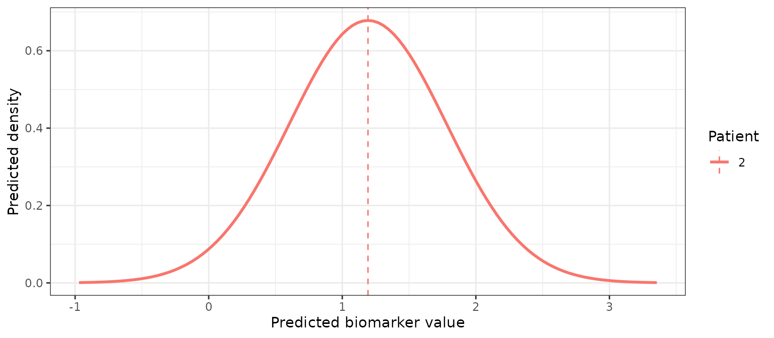

Predicted density of patient 2's log bilirubin one year after year 5, a single bell-shaped curve with a dashed line at its most likely value, near 1.2.

Step 5: plotting a patient’s risks

predictPlot() fixes the landmark and lets the window grow: it shows the biomarker history, the predicted future biomarker, and the risk of each event type as the horizon increases (event type 1 is death, event type 2 transplantation).

predictPlot(list(patient, patient), long_fit, survival_fit,
            prediction_time = 5, horizon = seq(0, 3, 0.5), time_variable = "year",
            survival_variable_all = list(), survival_trans_function = list())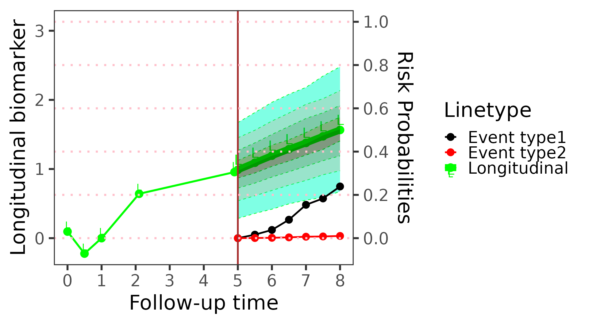

Prediction plot for patient 2 at year 5: the observed bilirubin history up to year 5, the predicted future bilirubin with widening uncertainty bands from year 5 to 8, and the predicted risk of the two event types growing with the horizon, death to about 0.25 by year 8 and transplantation staying near 0.

riskPlot() instead fixes the window, here one year, and moves the landmark, so each risk uses more of the history:

riskPlot(list(patient, patient), long_fit, survival_fit,
         prediction_time = c(1, 2, 3, 4, 5), bio_i = 1, horizon = 1, time_variable = "year",
         survival_variable_all = list(), survival_trans_function = list())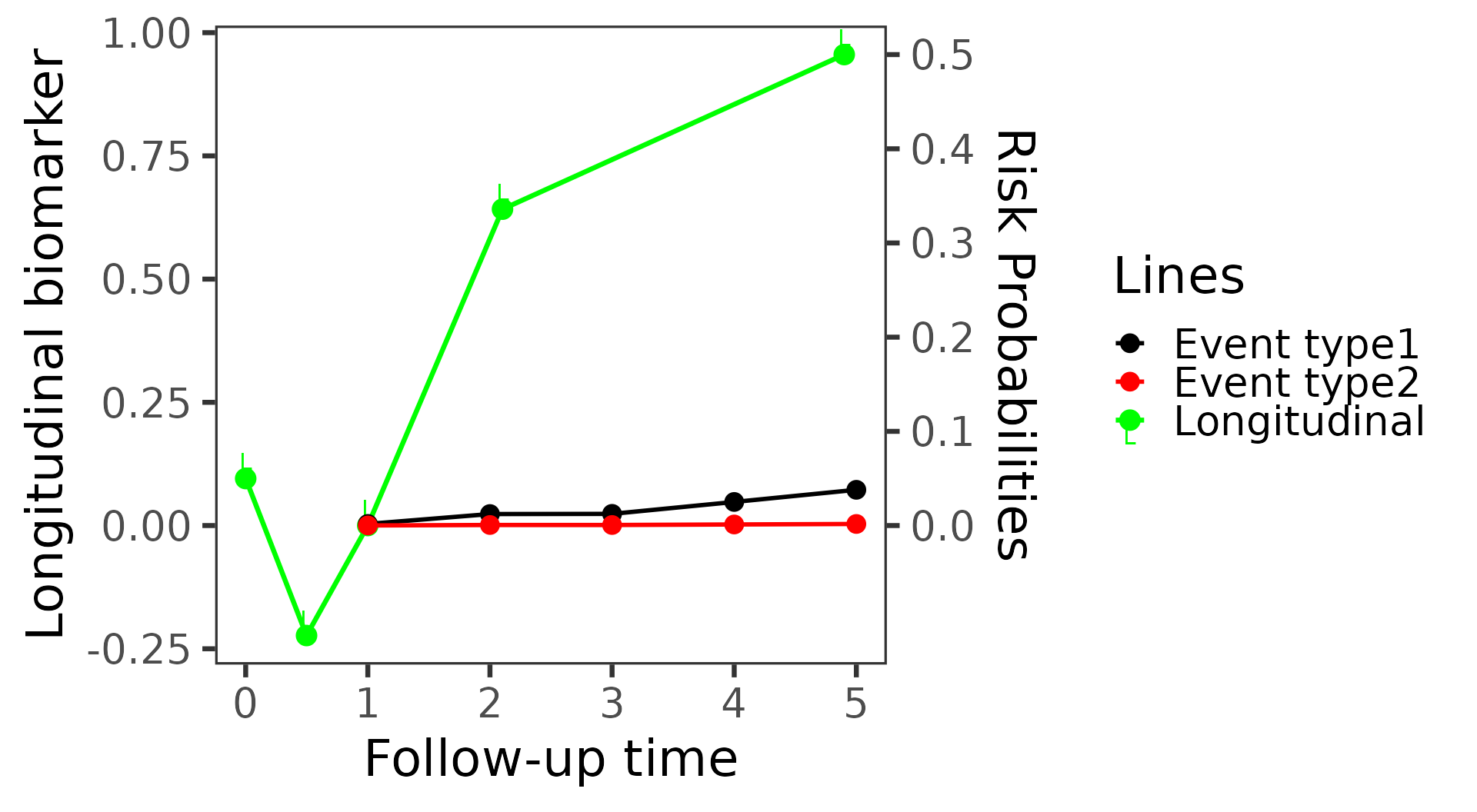

Patient 2's bilirubin history from year 0 to 5 together with the predicted one-year risks of the two event types at landmarks 1 to 5; the risk of death rises slowly as bilirubin increases, and the transplantation risk stays near 0.

Step 6: simulated futures with `simulateTrajectory()`

simulateTrajectory() draws complete futures from the model. With competing risks each draw has an event time and an event type, in the status4 column:

sims <- simulateTrajectory(list(patient, patient), long_fit, survival_fit,
                           prediction_time = 5, times = seq(5, 12, 0.5), time_variable = "year",
                           survival_variable_all = list(), survival_trans_function = list(),
                           n_sim = 500, seed = 1)
draws <- sims[!duplicated(sims$sim), ]
table(type = draws$status4, event = draws$event, useNA = "ifany")
#>       event
#> type     0   1
#>   0      0 413
#>   1      0  17
#>   <NA>  70   0

The cumulative incidence of each event type computed from the draws is a patient-specific version of the cifPlot() above:

plot(sims, which = "event")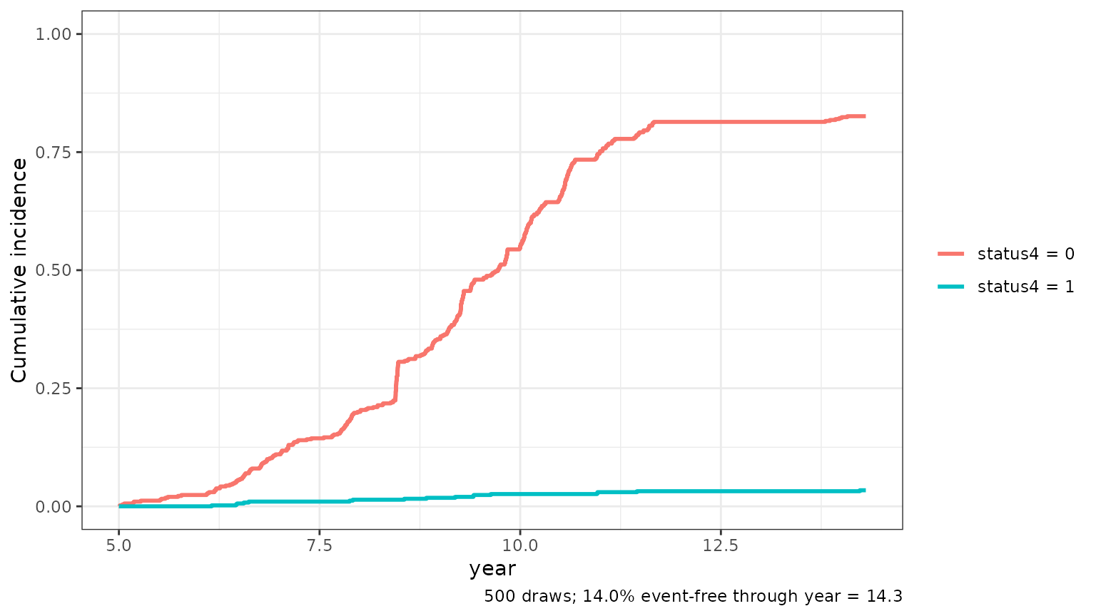

Cumulative incidence of death and transplantation for patient 2 after year 5, computed from 500 simulated event times: death rises to about 0.83 by year 14.3, mostly between years 8 and 11, and transplantation stays below 0.05.

Step 7: evaluating the predictions

performancePlot() and calibrationPlot() report the time-dependent AUC, the Brier score and the calibration of each event type separately; see the Plotting with BJM article for an example on held-out data.

Things to watch for

Two event types. The event-type model is a logistic regression, so BJM handles two competing event types. Combine rarer types, or model them one against the rest.
The coding of the event type decides which risk is risk_prob_1 (value 0, or the first factor level) and which is risk_prob_2.
Censored patients have an NA event type. They are used by the Cox model but not by the event-type model, and not by the biomarker models, which are fit on the patients with an event.
The event time in the event-type model must be a plain linear term (years, not log(years) or a spline): the predictions integrate over it.
The outcome columns are unknown for a new patient. Set years and status4 to NA in the prediction data, or leave status4 out.